Recurrent Neural Networks (RNNs) are a neural network architecture used for predicting sequence data. The most well known application of RNNs is in the field of Natural Language Processing. However, due to the complexity of actually implementing RNNs on text data (converting to one hot encoding, removing stopwords, and more) we will cover that in another post. This one will focus on how you can build and implement a simple, 3-layer Recurrent Neural Network architecture from scratch. In this post we’ll go over:

• An Introduction to Recurrent Neural Networks
  • Recurrent Neural Network Architecture
  • Recurrent Neural Network Applications
• File Organization for our RNN
• Building and Training the Recurrent Neural Network
  • Sigmoid Activation Function
  • Loss Calculating Function for the RNN
  • Calculating Layer Activations for the RNN
  • RNN Backpropagation
  • Training the Recurrent Neural Network
• Data Setup for Training and Testing the Recurrent Neural Network
  • Train/Test Split on Sequence Data
  • Setting up the Recurrent Neural Network
• Training and Testing the RNN on Sequence Data
  • Example of RNN on a Sine Function (Training Results)
  • Example of RNN on a Sine Function (Test Results)

Introduction to Recurrent Neural Networks

The simplest version of a Recurrent Neural Network is a three layer, fully connected neural network, which “recurs” itself in the middle layer. Normally nodes only pass their results forward. In the RNN architecture, nodes feed their results into their own input as well as passing them forward.

Recurrent Neural Network Architecture

The idea of recursion can be kind of scary. However, a Recurrent Neural Network architecture does not have to be scary. The image above shows what it really looks like we “unfold” a recurrent node/neuron. You can think of each “recurrence” as a step in a time series. We can control how many recurrence steps we take as a hyperparameter.

Recurrent Neural Network Applications

RNNs have many applications. They are most famous for being used to train on text data, but as I said above, they can be used to train on any sequence data. Examples of sequences could be the Sine function (which is what we’ll play with), waveform audio data (which looks sinusoidal), and the structure of DNA. Real world applications of RNNs on text data include language modeling, machine translation, and speech recognition.

File Organization for Our RNN

We’ll be building an RNN with two files. The files will be simple_rnn.py and test_simple_rnn.py. The simple_rnn.py function will contain the code to train the recurrent neural network. Everything needed to test the RNN and examine the output goes in the test_simple_rnn.py file. Check out the code on Github if anything is confusing.

Building and Training the Recurrent Neural Network

As we always do, we start our function by importing libraries. The only two libraries we’ll need for this are the math and numpy library. The math library is a built- in Python library, but numpy is not. We’ll need to install numpy. We can do so by using the below command in the terminal.

pip install numpy

import math
import numpy as np

After our imports, let’s set up our RNN Architecture. We need to set up the learning rate, sequence length, maximum number of training epochs, the dimension of the hidden and output layers, how many iterations back we want to go when doing back propagation, and the maximum and minimum values we’ll allow for our gradients.

# create RNN architecture
learning_rate = 0.0001
seq_len = 50
max_epochs = 25
hidden_dim = 100
output_dim = 1
bptt_truncate = 5 # backprop through time --> lasts 5 iterations
min_clip_val = -10
max_clip_val = 10

Sigmoid Activation Function

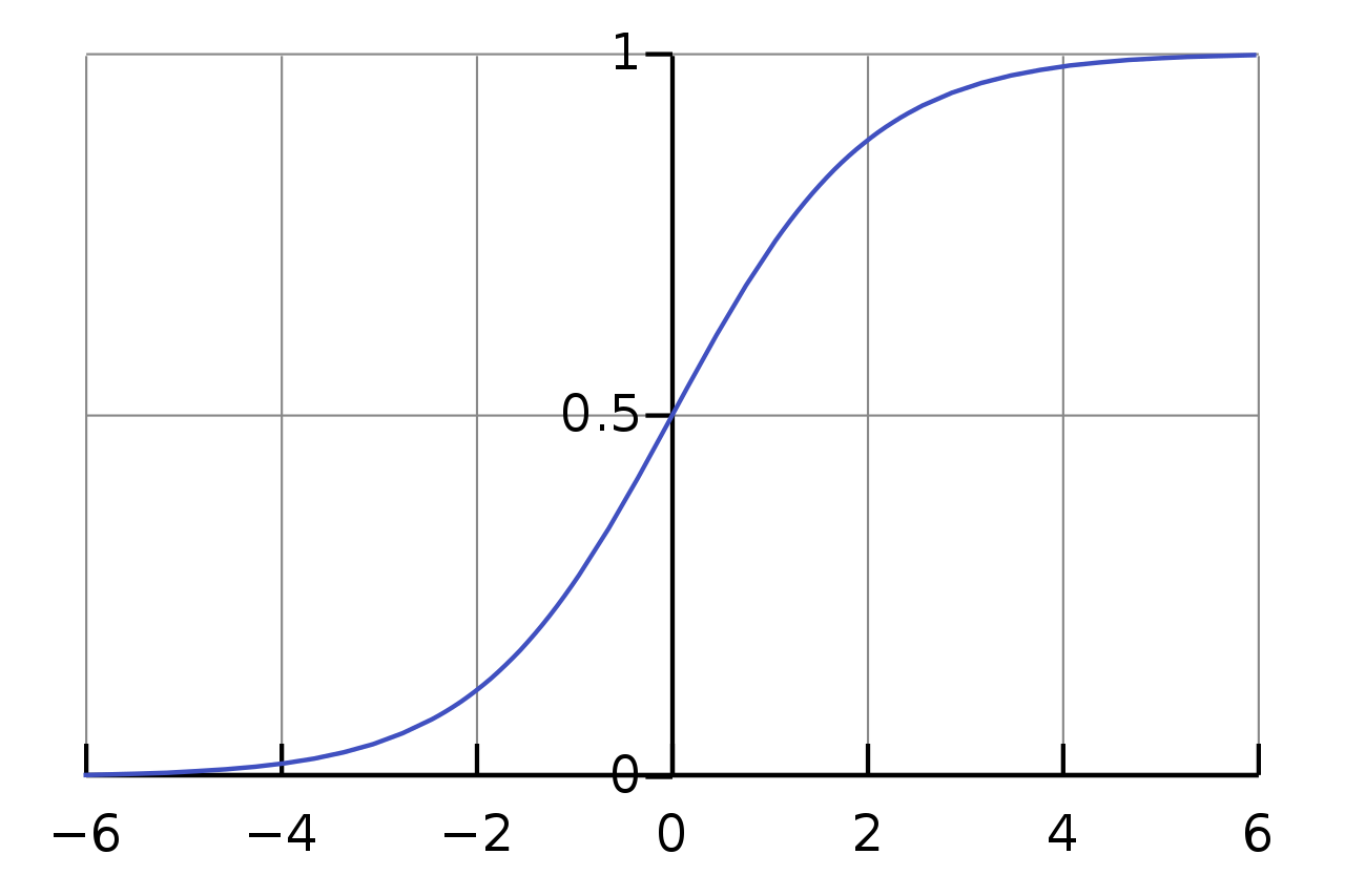
Logistic-curve – Sigmoid function – WikipediaThe sigmoid function is a classic activation function used for classification in neural networks. We first introduced this in an Introduction to Machine Learning: Logistic Regression. The sigmoid function takes one parameter, x, and returns the 1 divided by the sum of 1 and the exponential of x.

def sigmoid(x):
    return 1/(1+np.exp(-x))

Loss Calculating Function for the Recurrent Neural Network

The first function we’ll create for our RNN is a loss calculator. Our calculate_loss function will take five parameters: X, Y, U, V, and W. X and Y are the data and result matrices. U, V, and W are the weight matrices for the RNN. The U matrix represents the weights from the input layer to the hidden layer. The V matrix represents the weights from the hidden layer to the output layer. Finally, the W matrix represents the recurrent weights from the hidden layer to itself.

We initialize our loss to 0 before looping through each point of data. For each of the data points, we’ll initialize an x and y (lowercase this time) to represent the input and output of that data point. We will also initialize our previous activation to an array of zeros with size equal to the number of nodes in the hidden layer by 1. Then we’ll loop through each “time step” or recurrence in the sequence.

For each timestep, we’ll perform a forward pass. We initialize an input of 0s with a shape equal to our input, x. Then we define the input for that timestep to be equal to the value in the x at the index of that timestep. Now, we’ll create the activation by multiplying U with the input, multiplying W with the previous activation, and then summing them and taking the sigmoid output. With the activation calculated, we can calculate the output of our RNN as the dot product of V with the activation. Finally, we’ll want to set the previous activation to the current activation for the next entry in the sequence.

At the end of the sequence, we have the final output from that sequence, the final mulv variable. We’ll subtract that from the expected output, y, square it and divide by 2 to get our loss value for the datapoint. At the end of the loop, we’ll add that to the total loss. Finally, after we’ve looped through each entry in Y, we have a total loss. Which we will return along with the activation values. We’ll need these later.

def calculate_loss(X, Y, U, V, W):
    loss = 0.0
    for i in range(Y.shape[0]):
        x, y = X[i], Y[i]
        prev_activation = np.zeros((hidden_dim, 1)) # value of previous activation
        for timestep in range(seq_len):
            new_input = np.zeros(x.shape) # forward pass, done for each step in the sequence
            new_input[timestep] = x[timestep] # define a single input for that timestep
            mulu = np.dot(U, new_input)
            mulw = np.dot(W, prev_activation)
            _sum = mulu + mulw
            activation = sigmoid(_sum)
            mulv = np.dot(V, activation)
            prev_activation = activation
        # calculate and add loss per record
        loss_per_record = float((y - mulv)**2/2)
        loss += loss_per_record
    # calculate loss after first Y pass
    return loss, activation

Calculating Layer Activations for the RNN

Now that we’ve created a function to calculate the loss of the model, let’s create a function to get back the activation values of the layers. The layers we’re referring to here aren’t the three layers in the model, but rather the layers created by the recurrence relation of our recurrent neural network.

Our calc_layers function will take five parameters, x, U, V, W, and prev_activation. U, V, and W are the weight matrices just like above. x is the input matrix for this data point, and prev_activation is the previous activation for the final layer. We’ll begin our function by creating an empty layers list before looping through each timestep in the sequence.

In each timestep of the sequence we’ll start by creating an input similarly to the way we did in the loss function. We’ll create an array of zeros in the shape of x except for the index of the timestep which will be the corresponding value from the x matrix. Then we’ll create the activations from the U and W matrices. We multiply the U matrix by the input and the W matrix by the previous activation, sum them, and pass them through the sigmoid function to get the activation.

Now we multiply the weights for the output layer, V, and the activation matrix to get the final layer output values. Then we append the current and previous activation to the layers list we created earlier. At the end of the loop, we’ll replace the previous activation with the new activation and repeat. Finally, after looping through the whole sequence, we’ll return the layers, and the last outputs from each layer.

# takes x values and the weights matrices
# returns layer dictionary, final weights (mulu, mulw, mulv)
def calc_layers(x, U, V, W, prev_activation):
    layers = []
    for timestep in range(seq_len):
        new_input = np.zeros(x.shape)
        new_input[timestep] = x[timestep]
        mulu = np.dot(U, new_input)
        mulw = np.dot(W, prev_activation)
        _sum = mulw + mulu
        activation = sigmoid(_sum)
        mulv = np.dot(V, activation)
        layers.append({'activation': activation, 'prev_activation': prev_activation})
        prev_activation = activation
 
    return layers, mulu, mulw, mulv

RNN Truncated Backpropagation Through Time

Backpropagation is the function that updates the weights of a neural network. We need the loss and activation layer values that we created functions for above to do backpropagation. We’ll break the backpropagation for the RNN into three steps: setup, truncated backpropagation through time, and gradient trimming.

RNN Backpropagation Setup

Our backpropagation function will take eight parameters. It will take the input matrix, x, the weight matrices U, V, and W, the differential for the last layer, dmulv, the input values to the hidden layer, mulu, and mulw, and the list of layer activations, layers.

The first thing we’ll do in our RNN backpropagation is to set up the differentials. First, let’s set up the differentials for each layer, dU, dV, and dW. Then we’ll set up the differentials for each layer in the timestep, dU_t, dV_t, and dW_t. Next, we’ll set up the differentials for the truncated backpropagation through time, dU_i, and dW_i. We’ll set all of these differentials to a matrix of 0s in the shape of the U, V, and W matrices. Finally, we’ll set up the input weights of the hidden layer as the most recent sum of the U and V matrix weight outputs and the differential of the last layer.

def backprop(x, U, V, W, dmulv, mulu, mulw, layers):
    dU = np.zeros(U.shape)
    dV = np.zeros(V.shape)
    dW = np.zeros(W.shape)
   
    dU_t = np.zeros(U.shape)
    dV_t = np.zeros(V.shape)
    dW_t = np.zeros(W.shape)
   
    dU_i = np.zeros(U.shape)
    dW_i = np.zeros(W.shape)
   
    _sum = mulu + mulw
    dsv = np.dot(np.transpose(V), dmulv)

Get Previous Hidden Layer Activation Differential

We need to calculate the differential for the previous activation of the hidden layer multiple times so we’ll factor it out into its own function. This function will take three parameters, the sum of the weight outputs, the differential from the output layer, and the weights layer. The function will get the differential of the sum by multiplying the sum of the weight outputs by its “inverse” from 1, and the differential from the output layer. Then we’ll create the differential of the hidden layer output by multiplying the differential of the sum by a matrix in the shape of the output layer differential. Finally, we’ll return the dot product of the hidden layer weights and the differential we created earlier.

    def get_previous_activation_differential(_sum, ds, W):
        d_sum = _sum * (1 - _sum) * ds
        dmulw = d_sum * np.ones_like(ds)
        return np.dot(np.transpose(W), dmulw)

Truncated Backpropagation Through Time

Truncated Backpropagation Through Time is the backpropagation method for Recurrent Neural Networks. Earlier we set a bptt_truncate value to set the number of timesteps back that we’ll go (in this case 5). For each timestep in the sequence length, we’ll start by getting the differential of the last layer in that time step by multiplying the last layer differential by the last layer activation. Then we’ll set up the differential of the last layer that we’ll change in this timestep, ds, as the dsv value we assigned in the set up.

After getting that differential, we’ll get the previous activation differential to pass into the truncated backpropagation. Now, we’ll do the truncated time series backpropagation by looping through each prior timestep. Within this inner loop, we’ll start by augmenting the last layer differential that we created earlier, and then getting the value of the previous activation in the previous timestep with that new differential. 

Next, we’ll create the differential for this recurrent timestep by getting the dot product of the hidden weights and the timestep’s previous activation. After this, we’ll do the same step we do in the forward pass by creating a new input for this recurrent timestep. This gives us the differential for the input layer for this recurrent timestep. Finally, we’ll increment the differential values for the hidden layer and the input layer with the differentials for the recurrent timestep.

    for timestep in range(seq_len):
        dV_t = np.dot(dmulv, np.transpose(layers[timestep]['activation']))
        ds = dsv
        dprev_activation = get_previous_activation_differential(_sum, ds, W)
       
        for _ in range(timestep-1, max(-1, timestep-bptt_truncate-1), -1):
            ds = dsv + dprev_activation
            dprev_activation = get_previous_activation_differential(_sum, ds, W)
            dW_i = np.dot(W, layers[timestep]['prev_activation'])
           
            new_input = np.zeros(x.shape)
            new_input[timestep] = x[timestep]
            dU_i = np.dot(U, new_input)
           
            dU_t += dU_i
            dW_t += dW_i

Taking Care of Exploding Gradients

Phew, that was a huge, possibly confusing section. Now that we’ve taken care of the truncated backpropagation through time for the recurrent hidden layer, let’s do something easier. We need to take care of exploding gradients so that our model will be more likely to converge. All we do is make sure that the maximum and minimum values of each of the differentials for the weight layers isn’t larger or smaller than the boundaries we set in the setup.

        # take care of possible exploding gradients
        if dU.max() > max_clip_val:
            dU[dU > max_clip_val] = max_clip_val
        if dV.max() > max_clip_val:
            dV[dV > max_clip_val] = max_clip_val
        if dW.max() > max_clip_val:
            dW[dW > max_clip_val] = max_clip_val
       
        if dU.min() < min_clip_val:
            dU[dU < min_clip_val] = min_clip_val
        if dV.min() < min_clip_val:
            dV[dV < min_clip_val] = min_clip_val
        if dW.min() < min_clip_val:
            dW[dW < min_clip_val] = min_clip_val
       
    return dU, dV, dW

Full Truncated Backpropagation Through Time Method

Here’s the full code for the truncated backpropagation through time function.

def backprop(x, U, V, W, dmulv, mulu, mulw, layers):
    dU = np.zeros(U.shape)
    dV = np.zeros(V.shape)
    dW = np.zeros(W.shape)
   
    dU_t = np.zeros(U.shape)
    dV_t = np.zeros(V.shape)
    dW_t = np.zeros(W.shape)
   
    dU_i = np.zeros(U.shape)
    dW_i = np.zeros(W.shape)
   
    _sum = mulu + mulw
    dsv = np.dot(np.transpose(V), dmulv)
   
    def get_previous_activation_differential(_sum, ds, W):
        d_sum = _sum * (1 - _sum) * ds
        dmulw = d_sum * np.ones_like(ds)
        return np.dot(np.transpose(W), dmulw)
   
    for timestep in range(seq_len):
        dV_t = np.dot(dmulv, np.transpose(layers[timestep]['activation']))
        ds = dsv
        dprev_activation = get_previous_activation_differential(_sum, ds, W)
       
        for _ in range(timestep-1, max(-1, timestep-bptt_truncate-1), -1):
            ds = dsv + dprev_activation
            dprev_activation = get_previous_activation_differential(_sum, ds, W)
            dW_i = np.dot(W, layers[timestep]['prev_activation'])
           
            new_input = np.zeros(x.shape)
            new_input[timestep] = x[timestep]
            dU_i = np.dot(U, new_input)
           
            dU_t += dU_i
            dW_t += dW_i
           
        dU += dU_t
        dV += dV_t
        dW += dW_t
       
        # take care of possible exploding gradients
        if dU.max() > max_clip_val:
            dU[dU > max_clip_val] = max_clip_val
        if dV.max() > max_clip_val:
            dV[dV > max_clip_val] = max_clip_val
        if dW.max() > max_clip_val:
            dW[dW > max_clip_val] = max_clip_val
       
        if dU.min() < min_clip_val:
            dU[dU < min_clip_val] = min_clip_val
        if dV.min() < min_clip_val:
            dV[dV < min_clip_val] = min_clip_val
        if dW.min() < min_clip_val:
            dW[dW < min_clip_val] = min_clip_val
       
    return dU, dV, dW

Training The Recurrent Neural Network

Everything is finally set up for creating the function to train our recurrent neural network. To train our RNN, we need seven parameters. These seven parameters are U, V, and W, the weight matrices, X, and Y, the training input data and results, and X_validation, and Y_validation, the validation input data and results. We’ll train our data for max_epochs number of epochs that we set up earlier.

Within each epoch, the first thing we’ll do is calculate the training and validation losses. Notice that we’ll just keep the previous activation from the training loss calculation. We’ll print out the training and validation losses of the epoch afterwards so we can keep track of how our training is going. The next thing we’ll do is loop through each data point.

For each data point, we’ll first make little x and y values. We’ll then create the layers list and initialize the previous activation. Next, we’ll calculate the layers with the calc_layers function we created earlier. Next we’ll get the difference of the prediction which we will then pass to the backpropagation function. The backpropagation function will return the differentials of the weight layers, and then update the weight layers.

# training
def train(U, V, W, X, Y, X_validation, Y_validation):
    for epoch in range(max_epochs):
        # calculate initial loss, ie what the output is given a random set of weights
        loss, prev_activation = calculate_loss(X, Y, U, V, W)
 
        # check validation loss
        val_loss, _ = calculate_loss(X_validation, Y_validation, U, V, W)
       
        print(f'Epoch: {epoch+1}, Loss: {loss}, Validation Loss: {val_loss}')
 
        # train model/forward pass
        for i in range(Y.shape[0]):
            x, y = X[i], Y[i]
            layers = []
            prev_activation = np.zeros((hidden_dim, 1))
           
            layers, mulu, mulw, mulv = calc_layers(x, U, V, W, prev_activation)
               
            # difference of the prediction
            dmulv = mulv - y
            dU, dV, dW = backprop(x, U, V, W, dmulv, mulu, mulw, layers)
           
            # update weights
            U -= learning_rate * dU
            V -= learning_rate * dV
            W -= learning_rate * dW
    return U, V, W

Data Setup for Training and Testing the RNN

We’ll need to install sklearn to get the RMSE (you don’t actually need to check the RMSE, but it is helpful for determining how good our model is). You can install sklearn with the following code:

pip install sklearn

This is our test_simple_rnn.py file. We’ll begin by importing numpy, matplotlib.pyplot as plt, and math. We need numpy and math for data manipulation and matplotlib.pyplot for plotting our series data. We’ll also import mean_squared_error from sklearn.metrics to check the root mean square error (RMSE) at the end of the training. Finally, we’ll import the train and sigmoid function as well as the hyperparameters for the hidden dimensions, sequence length, and output dimensions from the simple_rnn.py file we made.

import numpy as np
import matplotlib.pyplot as plt
import math
 
from sklearn.metrics import mean_squared_error
 
from simple_rnn import train, hidden_dim, seq_len, sigmoid, output_dim

Train/Test Split on Sequence Data for the RNN

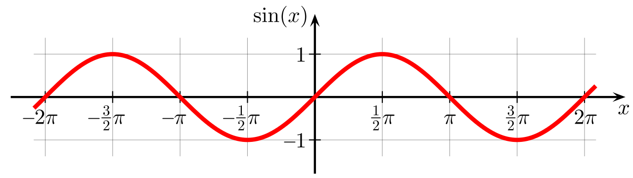
We’ll be training our Recurrent Neural Network on a sine wave. Sine waves are sequence data that oscillate with a period of 2$pi. After getting the sine wave data, we’ll set up our training and testing data. Let’s initialize two empty lists, X for the input sequence data, and Y for the next data point in the sequence.

We’ll set each datapoint of X as 50 contiguous points in the series and each datapoint of Y as the next datapoint in the sine wave. We’ll set the training data to the first 100 points, and the validation data as the next 50. After creating the lists, we’ll turn them into matrices using np.expand_dims.

sin_wave = np.array([math.sin(x) for x in range(200)])
# training data
X = []
Y = []
num_records = len(sin_wave) - seq_len # 150
 
# X entries are 50 data points
# Y entries are the 51st data point
for i in range(num_records-50):
    X.append(sin_wave[i:i+seq_len])
    Y.append(sin_wave[i+seq_len])
 
X = np.expand_dims(np.array(X), axis=2) # 100 x 50 x 1
Y = np.expand_dims(np.array(Y), axis=1) # 100 x 1
 
# validation data
X_validation = []
Y_validation = []
for i in range(num_records-seq_len, num_records):
    X_validation.append(sin_wave[i:i+seq_len])
    Y_validation.append(sin_wave[i+seq_len])
 
X_validation = np.expand_dims(np.array(X_validation), axis=2)
Y_validation = np.expand_dims(np.array(Y_validation), axis=1)

Setting Up the Recurrent Neural Network Architecture

Now that we’ve set up the training and validation data, let’s set up the Recurrent Neural Network Architecture. All we’re going to do here is initialize the U, V, and W matrices, the weights for the input to hidden layer, hidden to output layer, and the hidden to hidden layer respectively. Notice that I set np.random.seed beforehand. This is to make our results reproducible. Each time we run the test with the same seed we will get the same result. The numpy.random library’s seed setting function is the same as the one we went over for the Python random library.

np.random.seed(12161)
U = np.random.uniform(0, 1, (hidden_dim, seq_len)) # weights from input to hidden layer
V = np.random.uniform(0, 1, (output_dim, hidden_dim)) # weights from hidden to output layer
W = np.random.uniform(0, 1, (hidden_dim, hidden_dim)) # recurrent weights for layer (RNN weigts)

Training and Testing the RNN on Sequence Data

Before we can test our RNN, we have to train it. Earlier in our test_simple_rnn.py file we imported the train function from the simple_rnn.py file. Now we’ll train our function on the randomized weight layers, and the inputs and results that we created from the sine function.

U, V, W = train(U, V, W, X, Y, X_validation, Y_validation)

Example of RNN on a Sine Function (Training Fit):

To get the predictions on our data, we have to loop through each datapoint, and do a forward pass using the U, V, and W weights we trained earlier. For each datapoint, we do almost the same thing we did in calculate_loss to get the predictions. We go through the sequence and take each dot product for the weights layers, getting the activation, and replacing the previous activation. After each pass of the sequence data, we’ll append the final output activation to the predictions.

# predictions on the training set
predictions = []
for i in range(Y.shape[0]):
    x, y = X[i], Y[i]
    prev_activation = np.zeros((hidden_dim,1))
    # forward pass
    for timestep in range(seq_len):
        mulu = np.dot(U, x)
        mulw = np.dot(W, prev_activation)
        _sum = mulu + mulw
        activation = sigmoid(_sum)
        mulv = np.dot(V, activation)
        prev_activation = activation
    predictions.append(mulv)
 
predictions = np.array(predictions)
 
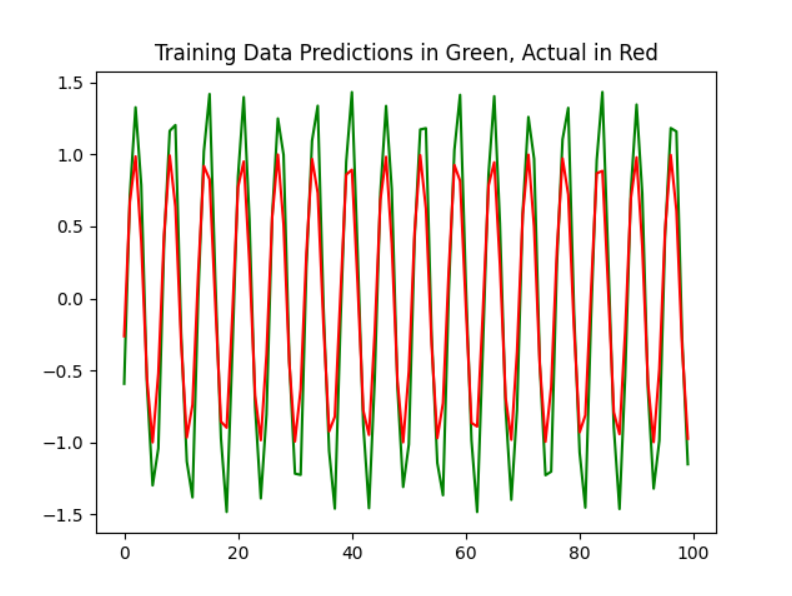
plt.plot(predictions[:, 0,0], 'g')
plt.plot(Y[:, 0], 'r')
plt.title("Training Data Predictions in Green, Actual in Red")
plt.show()

The last thing we do when running the data is plot the training data in green and the actual data in red. We should see an image like the one below:

Example of RNN on a Sine Function (Test Fit):

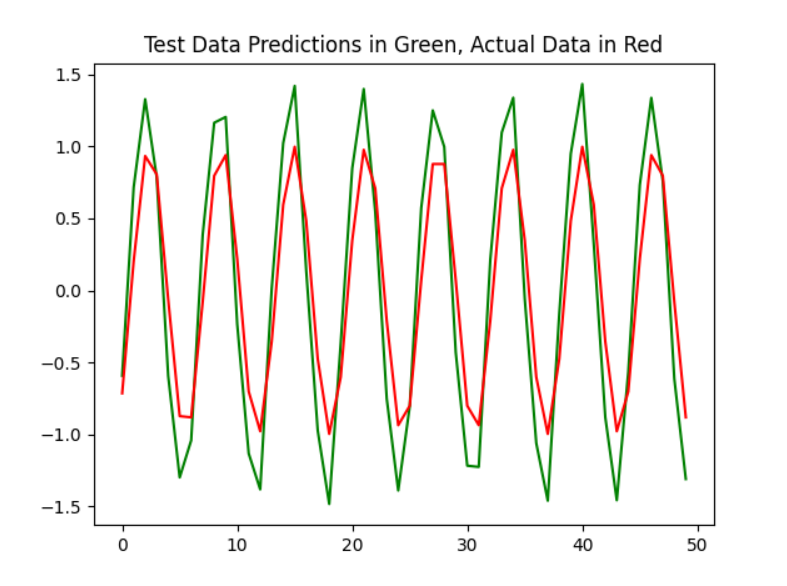
To test the Recurrent Neural Network, we’ll do the exact same thing we did to plot the training data, except instead of using the training data, we’ll use the validation data.

# predictions on the validation set
val_predictions = []
for i in range(Y_validation.shape[0]):
    x, y = X[i], Y[i]
    prev_activation = np.zeros((hidden_dim,1))
    # forward pass
    for timestep in range(seq_len):
        mulu = np.dot(U, x)
        mulw = np.dot(W, prev_activation)
        _sum = mulu + mulw
        activation = sigmoid(_sum)
        mulv = np.dot(V, activation)
        prev_activation = activation
    val_predictions.append(mulv)
 
val_predictions = np.array(val_predictions)
 
plt.plot(val_predictions[:, 0,0], 'g')
plt.plot(Y_validation[:, 0], 'r')
plt.title("Test Data Predictions in Green, Actual Data in Red")
plt.show()

Checking RMSE

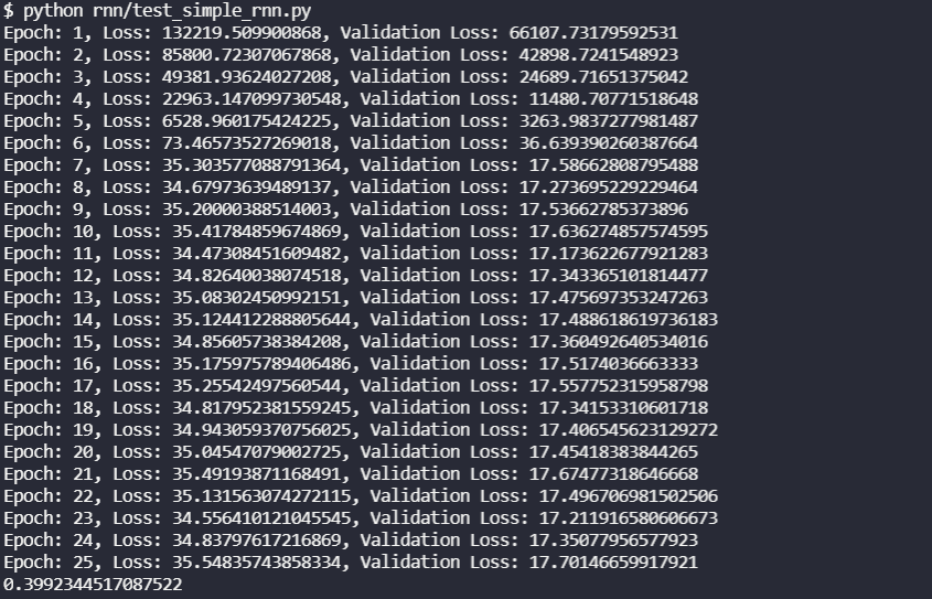
The last thing we’ll do to check how our model is doing is check the root mean squared error of our function. All we need to do for this is run the mean_squared_error function on the validation data results and the validation predictions and then take a square root.

# check RMSE
rmse = math.sqrt(mean_squared_error(Y_validation[:,0], val_predictions[:, 0, 0]))
print(rmse)

Our output, including the training and validation losses, should look like the image below.

Further Reading

• Prims Algorithm in Python
• Build Your Own AI Text Summarizer in Python
• Create a Neural Network from Scratch with Python 3
• Kruskal’s Algorithm in Python
• Build a GRU RNN with Keras

I run this site to help you and others like you find cool projects and practice software skills. If this is helpful for you and you enjoy your ad free site, please help fund this site by donating below! If you can’t donate right now, please think of us next time.