Welcome to our fourth installment on Algorithms and Data Structures in Python. If you haven’t read up on Stacks, Queues, and Dequeues and Linked Lists and Binary Trees you’ll want to read those to get a grasp on some simpler data structures we’ll be using and trees before we cover tree/graph traversals. Why am I using the terms tree and graph interchangeably? A tree is simply a one-directional graph.
There’s two main graph traversal algorithms: Breadth First Search (BFS) and Depth First Search (DFS). Depth First Search also has three traversal patterns – pre-order, in-order, and post-order. These traversal patterns have to do with the order in which we perform operations (in our case print) on the current node compared to its left and right children. Preorder prints the current node first. Inorder prints the current node in between the left and right nodes. Postorder prints the current node after its children node. Breadth First Search is sometimes also called “level-order search” because we are searching by each level in the tree.
Before we get into how to run these algorithms, let’s take a look at the graph we’ll work with here:

The adjacency list representation of this graph looks like:
graph = {
    0: [2],
    1: [2, 3],
    2: [0, 1, 6],
    3: [1, 5, 7],
    4: [7],
    5: [3],
    6: [2, 7],
    7: [3, 4, 6]
}
From our adjacency list we can tell that node 0 is only connected to node 2. Node 1 is connected to nodes 2, and 3. Node 2 is connected to nodes 0, 1, and 6. Node 3 is connected to nodes 1, 5, and 7. Node 4 is only connected to node 7. Node 5 is only connected to node 3. Node 6 is connected to nodes 2 and 7. Node 7 is connected to nodes 3, 4, and 6. Check for yourself that this corresponds directly to our undirected graph above.
Breadth First Search (BFS)
Let’s start with Breadth First Search or “level-order” search. BFS is an algorithm in which we traverse our tree/graph by “level”. This means that each node on the same level gets processed before the nodes on the level below it. A “level” is a measure of distance from the root node. For our example above, if we start with node 0, node 2 is on “level 1” because it’s one step away from node 0 while nodes 1 and 6 are on “level 2” because they are two steps away from node 0.
A BFS algorithm only requires two parameters: a graph in the form of an adjacency list and a starting node. An adjacency list is simply a dictionary in which each key is a node in the graph and has a corresponding value that is a list of adjacent nodes. For this example, we’ll be working with an undirected graph, that means that each “connection” between the nodes goes both ways.
Now let’s create our BFS algorithm. Our function will take two parameters, a graph and a starting node. The first thing we’ll do in our function is to set the list of visited nodes and a queue of nodes to visit. We’ll initialize both of these with the starting node. While the queue is not empty, we pop the first value from the queue and set that as our operating node. For this example, the operation is simply printing the node.
Once we’re done with the current node, we’ll check its neighbors and if the neighboring node is not yet in the list of visited nodes, we’ll append it to the queue and the list of visited nodes. As we loop through the queue, we’ll eventually cover every node and the ones next to it. The print statements for the visited nodes and the queue are unnecessary, but I’ve chosen to put them in here to give a little more insight into what’s going on in this algorithm.
def bfs(graph, starting_node):
visited = [starting_node]
queue = [starting_node]
while queue:
node = queue.pop(0)
print(f"Current Node: {node}")
print(f"Visited Nodes: {visited}")
for neighbor in graph[node]:
if neighbor not in visited:
visited.append(neighbor)
queue.append(neighbor)
print(f"Queue: {queue}")
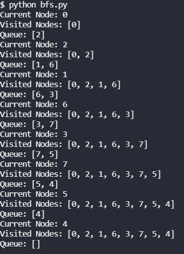
bfs(graph, 0)Once we run this BFS algorithm on our graph, starting with node 0, we should get an output like the one below. The final list of visited nodes is the result of our breadth first search on this graph.
Depth First Search (DFS)
BFS processes nodes by level, DFS processes nodes by doing an exhaustive search. It goes down a path in the graph until it can’t go down that path anymore, then begins processing. DFS can be implemented in both a recursive and a non-recursive (iterative) fashion. Due to its iterative nature, the non-recursive implementation of DFS can only be implemented as a preorder DFS. In this article we’ll cover how to implement the iterative form of DFS on the same graph we performed BFS on.
We will start out our iterative DFS algorithm in pretty much the same way we started our Breadth First Search. We need two parameters, the graph and the starting node. The first thing we’ll do is create a list of visited nodes, and this time instead of a queue, we will instantiate a stack. While our stack is not empty, we’ll pop the last element and print the current node.
Once we’re done with our operation on the current node (printing), we’ll go to its neighbors and check to see if the neighbors have been processed yet or are in the stack to be processed. Each neighboring node that hasn’t been processed or marked for processing is put onto the stack. As we loop through the graph, each node will have its turn in the stack based on how far away it is from the starting node.
def dfs_iterative(graph, starting_node):
    visited = [starting_node]
    stack = [starting_node]
    while stack:
        node = stack.pop()
        print(f"Current Node: {node}")
        if node not in visited:
            visited.append(node)
        print(f"Visited Nodes: {visited}")
        for neighbor in graph[node]:
            if neighbor not in visited and neighbor not in stack:
                stack.append(neighbor)
        print(f"Stack: {stack}")

dfs_iterative(graph, 0)
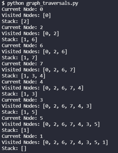
Once we run this, we should see an output like the following. When we start at 0, this time we’ll go all the way down to the furthest node – 4 – before we come back up. Node 4 will back us up to node 7, and instead of backing up to node 6, we’ll go to node 3 because 6 has already been processed. From node 3 we’ll go to 5 and 1. It may be slightly counter-intuitive that we visit 1 last since it could be visited from 2, but because DFS is an exhaustive search, it goes all the way down to the furthest nodes first. This exhaustive search is facilitated by the use of a stack and the way our adjacency list is structured.
Just for fun, if we reverse the order in which we list our nodes in the adjacency list, we’ll see a totally different DFS output. Note that this is still the same graph, we’re only changing the adjacency list representation of it.
graph = {
    0: [2],
    1: [3, 2],
    2: [6, 1, 0],
    3: [7, 5, 1],
    4: [7],
    5: [3],
    6: [7, 2],
    7: [6, 4, 3]
}

Why is this output different? Because we’ve changed the way the stack is structured. Now, when we get to node 2, we’re actually going to visit node 1 and traverse all the way through that before we visit node 6. To learn more, feel free to reach out to me @yujian_tang on Twitter, follow the blog, or join our Discord.
I run this site to help you and others like you find cool projects and practice software skills. If this is helpful for you and you enjoy your ad free site, please help fund this site by donating below! If you can’t donate right now, please think of us next time.
