Categories
level 3 python NLP The Text API

Using AI to Analyze COVID Headlines Over Time

We’re coming up on the second anniversary of the COVID-19 pandemic in America. There’s been a bunch of different variants, the CDC has shifted its stance at least 20 times, and the mask and vaccine protests rage on. Given all of this, I thought it would be interesting to analyze what the news has been saying about COVID over these last two years. In this post we will:

  • Download News Headlines from 2020 and 2021
  • Extract Headlines About COVID with AI
    • Setup requests to extract COVID headlines
    • Load and transform raw archived headline data from the NY Times
    • Extraction of COVID headlines using AI
  • Use AI to Get COVID Headlines Sentiments
    • Setup asynchronous polarity value extraction
    • Load up AI extracted COVID headlines to send to the API
    • Asynchronously send requests to get sentiment values for headlines
  • Plot COVID Headline Sentiments for 2020 and 2021 – see Sentiment Graphs Here
    • A table of the number of COVID headlines per month
    • Graphing sentiment polarity values for each headline
    • Graphing monthly, yearly, and total sentiment values 
    • Avoiding an asynchronous looping RuntimeError
    • The graph of average sentiment values of COVID per month since 2020
  • Create a Word Cloud of COVID Headlines for 2020 and 2021 – see Word Clouds Here
    • Moving the parse function to a common file
    • Code to create a word cloud
    • Loading the file and creating word clouds of COVID headlines
  • Use NLP to Find the Most Common Phrases in COVID Headlines So Far
    • Moving the base API endpoint and headers to a common file
    • Setting up requests to get most common phrases
    • Creating the requests to get most common phrases for each month
    • Calling the most common phrases API
    • The most common phrases in each month of COVID headlines
  • Summary of using AI to analyze COVID headlines over time

To follow along all you need is to get two free API keys, one from the NY Times, and one from The Text API, and install the requests, aiohttp, and wordcloud libraries. To install the libraries, you can simple run the following code in your terminal or command line:

pip install requests wordcloud aiohttp

Download News Headlines from 2020 and 2021

The first thing we need to do is download our news headlines. This is why we need the NY Times API. We’re going to use the NY Times to download their archived headlines from 2020 to 2021. We won’t go through all the code to do that in this section, but you can follow the guide on How to Download Archived News Headlines to get all the headlines. You’ll need to download each month from 2020 to 2021 to follow this tutorial. If you want, you can also get the headlines for December 2019 when COVID initially broke out.

Extract Headlines about COVID with AI

After we have the downloaded news headlines we want to extract the ones that contain “COVID” in their title. We’re going to use The Text API to do this. The first thing we’ll need to do is set up our API requests and our map of month to month number as we did when we downloaded the headlines. Then we need to load and transform the JSON data into usable headline data. Finally, we’ll send our API requests and get all of the headlines from January 2020, through December 2021 that contain COVID in their headlines.

Setup Requests for COVID Headline Extraction with AI

Since we’re using a Web API to handle our extraction, the first thing we’ll need to do is set up sending API requests. We’ll start by importing the requests and json library. Then we’ll import the API key we got from The Text API earlier as well as the URL endpoint, “https://app.thetextapi.com/text/”. We need to set up the actual headers and the keyword endpoint URL. The headers will tell the server that we’re sending JSON content and pass the API key. Finally, we’ll set up a month dictionary so we can map month numbers to their names. This is for loading the JSON requests.

import requests
import json
 
from config import thetextapikey, text_url
 
headers = {
    "Content-Type": "application/json",
    "apikey": thetextapikey
}
keyword_url = text_url+"sentences_with_keywords"
 
month_dict = {
    1: "January",
    2: "February",
    3: "March",
    4: "April",
    5: "May",
    6: "June",
    7: "July",
    8: "August",
    9: "September",
    10: "October",
    11: "November",
    12: "December"
}

Load and Transform Raw Data into Headlines and Text

Now that we’ve set up our requests, let’s load up our headlines. We’ll create a simple load_headlines file with two parameters, year, and month. First, we’ll open up the file and headlines. Replace <path to folder> with the path to your folder. From here, we’re going to create an empty string and empty list so we can loop through each entry and append the main and print headlines that go with each entry.

In our loop, we’ll have to check the print_headline for each entry because sometimes it is empty. We will then check the last character of the print headline and turn it into a period if it’s punctuation. We’ll also check the last character of the main headline and get rid of it if it’s punctuation. We do this because we’re going to get all the sentences that contain the word COVID with our AI keyword extractor.

If the print headline exists, we’ll concatenate the main headline, a comma, and then the print headline and a space (for readability and separability) with the existing headlines text. If the print headline doesn’t exist, we’ll just concatenate the main headline. Else, if the length of the headlines text is greater than 3000, we’ll append the lowercase version to the headlines list and clear the string.

It doesn’t have to be 3000, choose this number based on your internet speed, the faster your internet, the higher number of characters you can send. We use these separate headlines to ensure the connection doesn’t timeout. At the end of the function, return the list of headlines strings.

# load headlines from a month
# lowercase all of them
# search for covid
def load_headlines(year, month):
    filename = f"<path to folder>\\{year}\\{month_dict[month]}.json"
    with open(filename, "r") as f:
        entries = json.load(f)
    hls = ""
    hls_to_send = []
    # organize entries
    for entry in entries:
        # check if there are two headlines
        if entry['headline']["print_headline"]:
            if entry['headline']["print_headline"][-1] == "!" or entry['headline']["print_headline"][-1] == "?" or entry['headline']["print_headline"][-1] == ".":
                hl2 = entry['headline']["print_headline"]
            else:
                hl2 = entry['headline']["print_headline"] + "."
            # append both headlines
            if entry['headline']["main"][-1] == "!" or entry['headline']["main"][-1] == "?" or entry['headline']["main"][-1] == ".":
                hl = entry['headline']["main"][:-1]
            else:
                hl = entry['headline']["main"]
            hls += hl + ", " + hl2 + " "
        elif entry['headline']['main']:
            if entry['headline']["main"][-1] == "!" or entry['headline']["main"][-1] == "?" or entry['headline']["main"][-1] == ".":
                hl = entry['headline']["main"]
            else:
                hl = entry['headline']["main"] + "."
            hls += hl + " "
        # if hls is over 3000, send for kws
        if len(hls) > 3000:
            hls_to_send.append(hls[:-1].lower())
            hls = ""
    return(hls_to_send)

Extraction of COVID from Headlines using an NLP API

Now that we have the sets of headlines to send to the keyword extraction API, let’s send them off. We’ll create a function that takes two parameters, the year and month. The first thing the function does is call the load_headlines function we created earlier to load the headlines. Then we’ll create an empty list of headlines to hold the COVID headlines.

Next, we’ll loop through each set of headlines and create a body that contains the headlines as text and the list of keywords we want to extract. In this case, just “covid”. Then, we’ll send a POST request to the keyword extraction endpoint. When we get the response back, we’ll load it into a dictionary using the JSON library. After it’s loaded, we’ll add the list corresponding to “covid” to the COVID headlines list. You can see what an example response looks like on the documentation page.
Finally, after we’ve sent all the sets of headlines off and gotten the responses back, we’ll open up a text file. We’ll loop through every entry in the COVID headlines list and write it to the text file along with a new line character. You can also send these requests asynchronously like we’ll do in the section below. I leave that implementation as an exercise for the reader.

def execute(year, month):
    hls = load_headlines(year, month)
    covid_headlines = []
    for hlset in hls:
        body = {
            "text": hlset,
            "keywords": ["covid"]
        }
        response = requests.post(keyword_url, headers=headers, json=body)
        _dict = json.loads(response.text)
        covid_headlines += _dict["covid"]
    with open(f"covid_headlines/{year}_{month}.txt", "w") as f:
        for entry in covid_headlines:
            f.write(entry + '\n')

Use AI to Get COVID Headline Sentiments 

Now that we’ve extracted the headlines about COVID using an AI Keyword Extractor via The Text API, we’ll get the sentiments of each headline. We’re going to do this by sending requests asynchronously for optimized speed.

Set Up Asynchronous Polarity Requests

As usual, the first thing we’re going to do is set up our program by importing the libraries we need. We’ll be using the json, asyncio, and aiohttp modules as well as The Text API API key. After our imports, we’ll create headers which will tell the server that we’re sending JSON data and pass it the API key. Then we’ll declare the URL that we’re sending our requests to, the text polarity API endpoint. Next, we’ll make two async/await functions that will handle the asynchronous calls and pool them.

The first of the async/await functions we’ll create will be the gather function. This function will take two parameters (although, you could also do this with one), one for the number of tasks, and the number of tasks. The asterisk in front of the tasks parameter just indicates a variable number. The first thing we’ll do in this function is create a Semaphore to handle the tasks. We’ll create an internal function that will use the created Semaphore object to asynchronously await a task. That’s basically it, at the end we’ll return all the gathered tasks.

The other function we’ll make will be a function to send an asynchronous POST request. This function will take four parameters, the URL or API endpoint, the connection session, the headers, and the body. All we’ll do is asynchronously wait for a POST call to the provided API endpoint with the headers and body using the passed in session object to complete. Then we’ll return the JSON version of that object.

import json
import asyncio
import aiohttp
 
from config import thetextapikey
 
headers = {
    "Content-Type": "application/json",
    "apikey": thetextapikey
}
text_url = "https://app.thetextapi.com/text/"
polarities_url = text_url + "text_polarity"
 
# configure async requests
# configure gathering of requests
async def gather_with_concurrency(n, *tasks):
    semaphore = asyncio.Semaphore(n)
    async def sem_task(task):
        async with semaphore:
            return await task
   
    return await asyncio.gather(*(sem_task(task) for task in tasks))
 
# create async post function
async def post_async(url, session, headers, body):
    async with session.post(url, headers=headers, json=body) as response:
        text = await response.text()
        return json.loads(text)

Now that we’ve set up our asynchronous API calls, let’s retrieve the actual headlines. Earlier, we saved the headlines in text files. The first thing we’re going to do in this section is create a parse function that will take two parameters, a year and a month. We’ll start off the function by opening up the file and reading it into an “entries” variable. Finally, we’ll just return the entries variable.

def parse(year, month):
    with open(f"covid_headlines/{year}_{month}.txt", "r") as f:
        entries = f.read()
    return entries

Asynchronously Send Requests to Extract Sentiment Values

With the headlines loaded and the asynchronous support functions set up, we’re reading to create the function to extract sentiment values from the COVID headlines. This function will take two parameters, the year and the month. The first thing we’ll do is load up the entries using the parse function created above. Then we’ll split each headline into its own entry in a list. Next, we’ll establish a connector object and a connection session.

Now, we’ll create the request bodies that go along with the headlines. We’ll create a request for each headline. We’ll also need an empty list to hold all the polarities as we get them. If we need to send more than 10 requests, we’ll have to split those requests up. This is so we don’t overwhelm the server with too many concurrent requests. 

Once we have the requests properly set up, the only thing left to do is get the responses from the server. If there were more than 10 requests that were needed, we’ll await the responses and then add them to the empty polarities list, otherwise we’ll just set the list values to the responses. After asynchronously sending all the requests and awaiting all the responses, we’ll close the session to prevent any memory leakage. Finally, we’ll return the now filled up list of polarities.

# get the polarities asynchronously
async def get_hl_polarities(year, month):
    entries = parse(year, month)
    all_hl = entries.split("\n")
    conn = aiohttp.TCPConnector(limit=None, ttl_dns_cache=300)
    session = aiohttp.ClientSession(connector=conn)
    bodies = [{
        "text": hl
    } for hl in all_hl]
    # can't run too many requests concurrently, run 10 at a time
    polarities = []
    # break down the bodies into sets of 10
    if len(bodies) > 10:
        bodies_split = []
        count = 0
        split = []
        for body in bodies:
            if len(body["text"]) > 1:
                split.append(body)
                count += 1
            if count > 9:
                bodies_split.append(split)
                count = 0
                split = []
        # make sure that the last few are tacked on
        if len(split) > 0:
            bodies_split.append(split)
            count = 0
            split = []
        for splits in bodies_split:
            polarities_split = await gather_with_concurrency(len(bodies), *[post_async(polarities_url, session, headers, body) for body in splits])
            polarities += [polarity['text polarity'] for polarity in polarities_split]
    else:
        polarities = await gather_with_concurrency(len(bodies), *[post_async(polarities_url, session, headers, body) for body in bodies])
        polarities = [polarity['text polarity'] for polarity in polarities]
    await session.close()
    return polarities

Plot COVID Headline Sentiments for 2020 and 2021

Now that we have created functions that will get us the sentiment values for the COVID headlines from 2020 to 2021, it’s time to plot them. Plotting the sentiments over time will give us an idea of how the media has portrayed COVID over time. Whether they have been optimistic or pessimistic about the outcome, some idea of what’s going on at large, and whether or not the general sentiment is good. See all the graphs here

Number of COVID Headlines Over Time

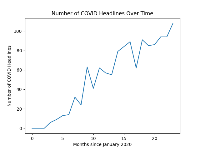
First let’s take a look at the number of COVID headlines over time.

MonthNYTimes Headlines About COVID
January 20200
February 20200
March 20200
April 20206
May 20209
June 202013
July 202014
August 202032
September 202024
October 202063
November 202041
December 202062
January 202157
February 202155
March 202179
April 202184
May 202189
June 202162
July 202191
August 202185
September 202186
October 202194
November 202194
December 2021108

Here’s the number of COVID headlines over time in graph format:

Graph Sentiment Polarity Values for Each Article

Now we’ve got everything set up, let’s plot the polarity values for each article. We’ll create a function which takes two parameters, the year and month. In our function, the first thing we’re going to do is run the asynchronous function to get the headline polarities for the year and month passed in. Note that this code is in the same file as the code in the section about using AI to get the sentiment of COVID headlines above.

Once we have the polarities back, we’ll plot it on a scatter plot using matplotlib. We’ll set up the title and labels so the plot looks good too. Then, we’ll save the plot and clear it. Finally, we’ll print out that we’re done plotting the month and year and return the list of polarity values we got back from the asynchronous API call.

# graph polarities by article
def polarities_graphs(year, month):
    polarities = asyncio.run(get_hl_polarities(year, month))
    plt.scatter(range(len(polarities)), polarities)
    plt.title(f"Polarity of COVID Article Headlines in {month_dict[month]}, {year}")
    plt.xlabel("Article Number")
    plt.ylabel("Polarity Score")
    plt.savefig(f"polarity_graphs/{year}_{month}_polarity.png")
    plt.clf()
    print(f"{month} {year} done")
    return polarities

Graph Monthly, Yearly, and Total Sentiment Polarity Values

We don’t just want to graph the polarity values for each article though, we also want to graph the sentiment values from each month and year. We’ll create a function that takes no parameters but gets the polarity values for each month in both years. Note that for some odd reason, there were exactly 0 mentions of COVID in the NYTimes headlines from January to March of 2020. Why? I don’t know, maybe there were mentions of “coronavirus” instead, but that’s out of the scope of this post and I’ll leave that as an exercise to you, the reader, to figure out.

This function will loop through both 2020 and 2021 as well as each of the first 12 numbers, we’ll have to add 1 to the month number because Python is 0 indexed. Once we loop through the years, we can plot the average polarity for each month. Once we’ve plotted both years, we will plot all the months on the same graph to get a full look at the COVID pandemic. Make sure to clear the figure between each plot for clarity.

# graph polarities by month
def polarities_month_graphs():
    total_polarities_over_time = []
    for year in [2020, 2021]:
        month_polarities = []
        for month in range(12):
            # skip over the first three months
            if year == 2020 and month < 3:
                month_polarities.append(0)
                continue
            polarities = polarities_graphs(year, month+1)
            month_polarities.append(sum(polarities)/len(polarities))
        total_polarities_over_time += month_polarities
        plt.plot(range(len(month_polarities)), month_polarities)
        plt.title(f"Polarity of COVID Article Headlines in {year}")
        plt.xlabel("Month")
        plt.ylabel("Polarity Score")
        plt.savefig(f"polarity_graphs/{year}_polarity.png")
        plt.clf()
    # get total graph for both years
    plt.plot(range(len(month_polarities)), month_polarities)
    plt.title(f"Polarity of COVID Article Headlines so far")
    plt.xlabel("Months since March 2020")
    plt.ylabel("Polarity Score")
    plt.savefig(f"polarity_graphs/total_polarity.png")
    plt.clf()

Avoiding RuntimeError: Event Loop is closed

If you run the above code, you’re going to get a RuntimeError: Event loop is closed after running the asyncio loop. There is a fix to this though. This isn’t an actual error with the program, this is an error with the loop shutdown. You can fix this with the code below. For a full explanation of what the error is and what the code does, read this article on the RuntimeError: Event loop is closed Fix.

"""fix yelling at me error"""
from functools import wraps
 
from asyncio.proactor_events import _ProactorBasePipeTransport
 
def silence_event_loop_closed(func):
    @wraps(func)
    def wrapper(self, *args, **kwargs):
        try:
            return func(self, *args, **kwargs)
        except RuntimeError as e:
            if str(e) != 'Event loop is closed':
                raise
    return wrapper
 
_ProactorBasePipeTransport.__del__ = silence_event_loop_closed(_ProactorBasePipeTransport.__del__)
"""fix yelling at me error end"""

Total Graph of average COVID Sentiment in NY Times Headlines from 2020 to 2021

Here’s the graph of the average COVID sentiment in NY Times Headlines from 2020 to 2021. Keep in mind that there were 0 headlines about COVID from January to March though, that’s why they’re at 0.

Create a Word Cloud of COVID Headlines for 2020 and 2021

Another way we can get insights into text is through word clouds. We don’t need AI to build word clouds, but we will use the AI extracted COVID headlines to build them. In this section we’re going to build word clouds for each month of COVID headlines since 2020. See all the word clouds here.

Moving the Parse Function to a Common File

One of the first things we’ll do is move the parse function we created earlier to a common file. We’re moving this to a common file because it’s being used by multiple modules and it’s best practice to not repeat code. We should now have a common.py file in the same folder as our polarity grapher file and word cloud creator file.

def parse(year, month):
    with open(f"covid_headlines/{year}_{month}.txt", "r") as f:
        entries = f.read()
    return entries

Code to Create a Word Cloud, Modified for COVID

We’ll use almost the same code we used to create a word cloud for the AI extracted COVID headlines as we did for creating a word cloud out of Tweets. We’re going to make a slight modification here though. We’re going to add “covid” to the set of stop words. We already know that each of the headlines contains COVID so it doesn’t add any insight for us to see in a word cloud.

from wordcloud import WordCloud, STOPWORDS
import matplotlib.pyplot as plt
import numpy as np
from PIL import Image
 
# wordcloud function
def word_cloud(text, filename):
    stopwords = set(STOPWORDS)
    stopwords.add("covid")
    frame_mask=np.array(Image.open("cloud_shape.png"))
    wordcloud = WordCloud(max_words=50, mask=frame_mask, stopwords=stopwords, background_color="white").generate(text)
    plt.imshow(wordcloud, interpolation='bilinear')
    plt.axis("off")
    plt.savefig(f'{filename}.png')

Load the File and Actually Create the Word Cloud from COVID Headlines

Now that we’ve created a word cloud function, let’s create the actual word cloud creation file. Notice that we’re importing the word cloud function here. I opted to create a second file for creating the COVID word clouds specifically, but you can also create these in the same file. This is just to follow orchestration pattern practices. In this file we’ll create a function that takes a year and a month, parses the COVID headlines from that month, and creates a word cloud with the text. Then we’ll loop through both 2020 and 2021 and each month that contains COVID headlines and create word clouds for each month.

from common import parse
from word_cloud import word_cloud
 
def make_word_cloud(year, month):
    text = parse(year, month)
    word_cloud(text, f"wordclouds/{year}_{month}.png")
   
for year in [2020, 2021]:
    for month in range(12):
        if year == 2020 and month < 3:
            continue
        make_word_cloud(year, month+1)

Use NLP to Find Most Common Phrases in COVID Headlines

Finally, as an additional insight to how COVID has been portrayed in the media over time, let’s also get the most common phrases used in headlines about COVID over time. Like extracting the headlines and getting their polarity, we’ll also be using AI to do this. We’ll use the most_common_phrases endpoint of The Text API to do this.

Moving the Base API Endpoint and Headers to the Common File

The first thing we’ll do in this section is modify the common.py file we created and moved parse to earlier. This time we’ll also move the base URL and headers to the common file. We’ll be using the same base API URL and headers as we did for getting the sentiment values and extracting the keywords.

from config import thetextapikey
 
text_url = "https://app.thetextapi.com/text/"
headers = {
    "Content-Type": "application/json",
    "apikey": thetextapikey
}

Setup the Requests to Get Most Common Phrases using AI

The first thing we’ll do in this file is our imports (as always). We’ll be importing the json and requests libraries to send requests and parse them. We’ll also need the headers, base API URL, and parse function. Why are we using requests instead of asynchronous calls? We could use asynchronous calls here, but it’s not necessary. You can opt to use them for practice if you’d like. Finally, we’ll also set up the most_common_phrases API endpoint.

import json
import requests
 
from common import headers, text_url, parse
 
mcps_url = text_url + "most_common_phrases"

Creating a Monthly Request Function with an NLP API

Now that we’ve set up our requests for the most common phrases, let’s make a function that will get the most common phrases for a specific month. This function will take two parameters, a year and a month. The first thing we’ll do is create a body to send to the API. Then we’ll call the API by sending a POST request to the most common phrases endpoint. When we get our response back, we’ll load it into a JSON dictionary and extract out the list of most common phrases. Finally, we’ll write the most common phrases to an appropriate file.

# get the mcps asynchronously
def get_hl_mcps(year, month):
    body = {
        "text": parse(year, month)
    }
    response = requests.post(mcps_url, headers=headers, json=body)
    _dict = json.loads(response.text)
    mcps = _dict["most common phrases"]
    with open(f"mcps/{year}_{month}_values.txt", "w") as f:
        f.write("\n".join(mcps))

Call the API to Get the Most Common Phrases for Each Month

Now that we’ve written the function will extract the most common phrases from each set of monthly COVID headlines, we can just call it. We’ll loop through both years, 2020 and 2021, and all the months after March of 2020. For each loop, we’ll call the function we created above, and we will end up with a set of text files that contains the 3 most common phrases in headlines each month.

for year in [2020, 2021]:
    for month in range(12):
        if year == 2020 and month < 3:
            continue
        get_hl_mcps(year, month+1)

Most Common Phrases in COVID Headlines for Each Month since 2020

These are the 3 most common phrases in COVID headlines that we got using AI. Each phrase is equivalent to a noun phrase.

Month3 Most Common Phrases
April 2020possible covidcritical covid casesweary e.m.s. crews
May 2020covid syndromecovid patientsnew covid syndrome
June 2020covid infectionsmany covid patientscovid warning
July 2020fake covid certificatescovid spikelocal covid deaths
August 2020covid testscovid parentingcovid cases
September 2020covid riskcovid restrictionsd.i.y. covid vaccines
October 2020covid survivorcovid survivorscovid cases
November 2020covid overloadcovid testscovid laxity
December 2020covid pandemiccovid patientscovid breach
January 2021covid vaccinecovid survivorscovid spike
February 2021covid vaccineu.s. covid deathsrecord covid deaths
March 2021covid vaccinecovid vaccinescovid vaccine doses
April 2021effective covid vaccinescovid shotcovid certificates
May 2021covid vaccinecovid aidcovid data
June 2021covid vaccinessevere covidcovid cases
July 2021covid tollcovid returncovid patients
August 2021covid shotcovid shotscovid surge
September 2021covid vaccine boosterscovid vaccine pioneerscovid tests
October 2021covid vaccine mandatescovid boosterscovid pill
November 2021covid vaccine shotscovid vaccine mandatecovid vaccine mandates
December 2021covid pillcovid vaccinescovid boosters

Summary of How to Use AI to Analyze COVID Headlines Since March 2020

In this post we learned how we can leverage AI to get insights into COVID headlines. First we learned how to use AI to extract headlines about COVID from the NY Times archived headlines. Then, we used AI to get sentiment values from those headlines and plot them. Next, we created word clouds from COVID headlines. Finally, we got the most common phrases from each set of monthly COVID headlines. 

I run this site to help you and others like you find cool projects and practice software skills. If this is helpful for you and you enjoy your ad free site, please help fund this site by donating below! If you can’t donate right now, please think of us next time.

Categories
APIs level 3 python NLP The Text API

Using NLP to Get Insights from Twitter

I’m interested in analyzing the Tweets of a bunch of famous people so I can learn from them. I’ve built a program that will do this by pulling a list of recent tweets and doing some NLP on them. In this post we’re going to go over:

  • Get all the Text for a Search Term on Twitter
  • NLP Techniques to Run on Tweets
    • Summarization
    • Most Common Phrases
    • Named Entity Recognition
    • Sentiment Analysis
  • Running all the NLP Techniques Concurrently
  • Further Text Processing
    • Finding the Most Commonly Named Entities
  • Orchestration
  • A Summary

To follow along you’ll need a free API key from The Text API and to install the requests and aiohttp library with the following line in your terminal:

pip install requests aiohttp

Overview of Project Structure

In this project we’re going to create multiple files and folders. We’re going to create a file for getting all the text called pull_tweets.py. We’ll create a totally separate folder for the text processing, and we’ll have three files in there. Those three files are async_pool.py for sending the text processing requests, ner_processing.py for further text processing after doing NER, and a text_orchestrator.py for putting the text analysis together.

Get all the Text for a Search Term on Twitter

We went over how to Scrape the Text from All Tweets for a Search Term in a recent post. For the purposes of this program, we’ll do almost the exact same thing with a twist. I’ll give a succinct description of what we’re doing in the code here. You’ll have to go read that post for a play-by-play of the code. This is the pull_tweets.py file.

First we’ll import our libraries and bearer token. Then we’ll set up the request and headers and create a function to search Twitter. Our function will check if our search term is a user or not by checking to see if the first character is the “@” symbol. Then we’ll create our search body and send off the request. When we get the request back, we’ll parse it into JSON and compile all the Tweets into one string. Finally, we’ll return that string.

import requests
import json
 
from twitter_config import bearertoken
 
search_recent_endpoint = "https://api.twitter.com/2/tweets/search/recent"
headers = {
    "Authorization": f"Bearer {bearertoken}"
}
 
# automatically builds a search query from the requested term
# looks for english tweets with no links that are not retweets
# returns the tweets
def search(term: str):
    if term[0] == '@':
        params = {
            "query": f'from:{term[1:]} lang:en -has:links -is:retweet',
            'max_results': 25
        }
    else:
        params = {
            "query": f'{term} lang:en -has:links -is:retweet',
            'max_results': 25
        }
    response = requests.get(url=search_recent_endpoint, headers=headers, params=params)
    res = json.loads(response.text)
    tweets = res["data"]
    text = ". ".join( for tweet in tweets])
    return text

NLP Techniques to Run on Tweets

There’s a ton of different NLP techniques we can run, we can do Named Entity Recognition, analyze the text for polarity, summarize the text, and much more. Remember what we’re trying to do here. We’re trying to get some insight from these Tweets. With this in mind, for this project we’ll summarize the tweets, find the most common phrases, do named entity recognition, and run sentiment analysis.

We’re going to run all of these concurrently with asynchronous API requests. In the following sections we’re just going to set up the API requests. The first thing we’ll do is set up the values that are constant among all the tweets. This is creating the async_pool.py file.

Setup Constants

Before we can set up our requests, we have to set up the constants for them. We’ll also do the imports for the rest of the async_pool.py function. First, we’ll import the asyncio, aiohttp, and json libraries. We’ll use the asyncio and aiohttp libraries for the async API calls later. We’ll also import our API key that we got earlier from The Text API.

We need to set up the headers for our requests. The headers will tell the server that we’re sending JSON data and also pass the API key. Then we’ll set up the API endpoints. The API endpoints that we’re hitting are the summarize, ner, most_common_phrases, and text_polarity API endpoints.

import asyncio
import aiohttp
import json
 
from .text_config import apikey
 
# configure request constants
headers = {
    "Content-Type": "application/json",
    "apikey": apikey
}
text_url = "https://app.thetextapi.com/text/"
summarize_url = text_url+"summarize"
ner_url = text_url+"ner"
mcp_url = text_url+"most_common_phrases"
polarity_url = text_url+"text_polarity"

Summarize the Tweets

We’ll set up a function to return these bodies so we can use them later. We only need one parameter for this function, the text that we’re going to send. The first thing we’ll do in this function is set up an empty dictionary. Next we’ll set up the body to send to the summarize endpoint. The summarize endpoint will send the text and tell the server that we want a proportion of 0.1 of the Tweets.

def configure_bodies(text: str):
    _dict = {}    
    _dict[summarize_url] = {
        "text": text,
        "proportion": 0.1
    }

Find Most Common Phrases

After setting up the summarization body, we will set up the most_common_phrases body. This request will send the text and set the number of phrases to 5.

    _dict[mcp_url] = {
        "text": text,
        "num_phrases": 5
    }

Named Entity Recognition

Now we’ve set up the summarization and most common phrases request bodies. After those, we’ll set up the NER request body. The NER request body will pass the text and tell the server that we’re sending an “ARTICLE” type. The “ARTICLE” type returns people, places, organization, locations, and times.

    _dict[ner_url] = {
        "text": text,
        "labels": "ARTICLE"
    }

Sentiment Analysis

We’ve now set up the summarization, most common phrases, and named entity recognition request bodies. Next, is the sentiment analysis or text polarity body. Those terms are basically interchangeable. This request will just send the text in the body. We don’t need to specify any other optional parameters here. We’ll return the dictionar we created after setting this body.

    _dict[polarity_url] = {
        "text": text
    }
    return _dict

Full Code for Configuring Requests

Here’s the full code for configuring the request bodies.

# configure request bodies
# return a dict of url: body
def configure_bodies(text: str):
    _dict = {}
    _dict[summarize_url] = {
        "text": text,
        "proportion": 0.1
    }
    _dict[ner_url] = {
        "text": text,
        "labels": "ARTICLE"
    }
    _dict[mcp_url] = {
        "text": text,
        "num_phrases": 5
    }
    _dict[polarity_url] = {
        "text": text
    }
    return _dict

Run All NLP Techniques Concurrently

For a full play-by-play of this code check out how to send API requests asynchronously. I’ll go over an outline here. This is almost the exact same code with a few twists. This consists of three functions, gather_with_concurrency, post_async, and pool.

First, we’ll look at the gather_with_concurrency function. This function takes two parameters, the number of concurrent tasks, and the list of tasks. All we’ll do in this function is set up a semaphore to asynchronously execute these tasks. At the end of the function, we’ll return the gathered tasks.

Next we’ll create the post_async function. This function will take four parameters, the url, session, headers, and body for the request. We’ll asynchronously use the session passed in to execute a request. We’ll return the text after getting the response back.

Finally, we’ll create a pool function to execute all of the requests concurrently. This function will take one parameter, the text we want to process. We’ll create a connection and a session and then use the configure_requests function to get the request bodies. Next, we’ll use the gather_with_concurrency and post_async function to execute all the requests asynchronously. Finally, we’ll close the session and return the summary, most common phrases, recognized named entities, and polarity.

# configure async requests
# configure gathering of requests
async def gather_with_concurrency(n, *tasks):
    semaphore = asyncio.Semaphore(n)
    async def sem_task(task):
        async with semaphore:
            return await task
   
    return await asyncio.gather(*(sem_task(task) for task in tasks))
 
# create async post function
async def post_async(url, session, headers, body):
    async with session.post(url, headers=headers, json=body) as response:
        text = await response.text()
        return json.loads(text)
   
async def pool(text):
    conn = aiohttp.TCPConnector(limit=None, ttl_dns_cache=300)
    session = aiohttp.ClientSession(connector=conn)
    urls_bodies = configure_bodies(text)
    conc_req = 4
    summary, ner, mcp, polarity = await gather_with_concurrency(conc_req, *[post_async(url, session, headers, body) for url, body in urls_bodies.items()])
    await session.close()
    return summary["summary"], ner["ner"], mcp["most common phrases"], polarity["text polarity"]

Full Code for Asynchronously Executing all NLP techniques

Here’s the full code for async_pool.py.

import asyncio
import aiohttp
import json
 
from .text_config import apikey
 
# configure request constants
headers = {
    "Content-Type": "application/json",
    "apikey": apikey
}
text_url = "https://app.thetextapi.com/text/"
summarize_url = text_url+"summarize"
ner_url = text_url+"ner"
mcp_url = text_url+"most_common_phrases"
polarity_url = text_url+"text_polarity"
 
# configure request bodies
# return a dict of url: body
def configure_bodies(text: str):
    _dict = {}
    _dict[summarize_url] = {
        "text": text,
        "proportion": 0.1
    }
    _dict[ner_url] = {
        "text": text,
        "labels": "ARTICLE"
    }
    _dict[mcp_url] = {
        "text": text,
        "num_phrases": 5
    }
    _dict[polarity_url] = {
        "text": text
    }
    return _dict
 
# configure async requests
# configure gathering of requests
async def gather_with_concurrency(n, *tasks):
    semaphore = asyncio.Semaphore(n)
    async def sem_task(task):
        async with semaphore:
            return await task
   
    return await asyncio.gather(*(sem_task(task) for task in tasks))
 
# create async post function
async def post_async(url, session, headers, body):
    async with session.post(url, headers=headers, json=body) as response:
        text = await response.text()
        return json.loads(text)
   
async def pool(text):
    conn = aiohttp.TCPConnector(limit=None, ttl_dns_cache=300)
    session = aiohttp.ClientSession(connector=conn)
    urls_bodies = configure_bodies(text)
    conc_req = 4
    summary, ner, mcp, polarity = await gather_with_concurrency(conc_req, *[post_async(url, session, headers, body) for url, body in urls_bodies.items()])
    await session.close()
    return summary["summary"], ner["ner"], mcp["most common phrases"], polarity["text polarity"]

Further Text Processing

After doing the initial NLP we’ll still get some text back. We can continue doing some NLP on the summarization, most common phrases, and the named entities. Let’s go back to what we’re trying to do – get insights. The summary will help us get a general idea, the most common phrases will tell us what the most commonly said things are, but the NER is a little too broad still. Let’s further process the NER by finding the most commonly named entities.

Most Commonly Named Entities

For a play-by-play of this code, read the post on how to Find the Most Common Named Entities of Each Type. I’m going to give a high-level overview here. We’re going to build two functions, build_dict to split the named entities into each type, and most_common to sort that dictionary.

The build_dict function will take one parameter, ners, a list of lists. We’ll start off this function by creating an empty dictionary. Then we’ll loop through the list of ners and add those to the dictionary based on whether or not we’ve seen the type and name of the ner.

The most_common function will take one parameter as well, ners, a list of lists. The first thing we’ll do with this function is call build_dict to create the dictionary. Then, we’ll initialize an empty dictionary. Next, we’ll loop through the dictionary and sort each list of NER types. Finally, we’ll add the most common names in each type to the initialized dictionary and return that.

# build dictionary of NERs
# extract most common NERs
# expects list of lists
def build_dict(ners: list):
    outer_dict = {}
    for ner in ners:
        entity_type = ner[0]
        entity_name = ner[1]
        if entity_type in outer_dict:
            if entity_name in outer_dict[entity_type]:
                outer_dict[entity_type][entity_name] += 1
            else:
                outer_dict[entity_type][entity_name] = 1
        else:
            outer_dict[entity_type] = {
                entity_name: 1
            }
    return outer_dict
 
# return most common entities after building the NERS out
def most_common(ners: list):
    _dict = build_dict(ners)
    mosts = {}
    for ner_type in _dict:
        sorted_types = sorted(_dict[ner_type], key=lambda x: _dict[ner_type][x], reverse=True)
        mosts[ner_type] = sorted_types[0]
    return mosts

Orchestration

Finally, we’ll orchestrate our functions. First, we’ll start by importing the asyncio library and the two functions we’ll need to orchestrate, pool, and most_common. We’ll create one function, orchestrate_text_analysis, which will take one parameter, text.

The first thing we’ll do in our orchestrator is get the summary, NERs, most common phrases, and text polarity using asyncio to execute the four NLP techniques concurrently. Then, we’ll do more text processing on the NERs. We’ll also replace the newlines in the summary to make it more readable. Finally, we’ll return the summary, most common entities, most common phrases, and sentiment.

import asyncio
 
from .async_pool import pool
from .ner_processing import most_common
 
def orchestrate_text_analysis(text:str):
    """Step 1"""
    # task to execute all requests
    summary, ner, mcp, polarity = asyncio.get_event_loop().run_until_complete(pool(text))
   
    """Step 2"""
    # do NER analysis
    most_common_ners = most_common(ner)
    summary = summary.replace("\n", "")
    return summary, most_common_ners, mcp, polarity

Summary

In this post we went over how to pull Tweets for a search term and transform that into a text. Then, we went over how to asynchronously call four APIs to run NLP on the Tweets. Next, we went over how to do some further text processing. Finally, we went over how to orchestrate the NLP on the text. I’ll be using this program to get insights from some people I want to be like on Twitter.

I run this site to help you and others like you find cool projects and practice software skills. If this is helpful for you and you enjoy your ad free site, please help fund this site by donating below! If you can’t donate right now, please think of us next time.

Categories
level 3 python

Build a Recurrent Neural Network from Scratch in Python 3

Recurrent Neural Networks (RNNs) are a neural network architecture used for predicting sequence data. The most well known application of RNNs is in the field of Natural Language Processing. However, due to the complexity of actually implementing RNNs on text data (converting to one hot encoding, removing stopwords, and more) we will cover that in another post. This one will focus on how you can build and implement a simple, 3-layer Recurrent Neural Network architecture from scratch. In this post we’ll go over:

Introduction to Recurrent Neural Networks

The simplest version of a Recurrent Neural Network is a three layer, fully connected neural network, which “recurs” itself in the middle layer. Normally nodes only pass their results forward. In the RNN architecture, nodes feed their results into their own input as well as passing them forward.

Recurrent Neural Network Architecture

Recurrent Neural Network Unfolded, Image from Wikipedia

The idea of recursion can be kind of scary. However, a Recurrent Neural Network architecture does not have to be scary. The image above shows what it really looks like we “unfold” a recurrent node/neuron. You can think of each “recurrence” as a step in a time series. We can control how many recurrence steps we take as a hyperparameter.

Recurrent Neural Network Applications

RNNs have many applications. They are most famous for being used to train on text data, but as I said above, they can be used to train on any sequence data. Examples of sequences could be the Sine function (which is what we’ll play with), waveform audio data (which looks sinusoidal), and the structure of DNA. Real world applications of RNNs on text data include language modeling, machine translation, and speech recognition.

File Organization for Our RNN

We’ll be building an RNN with two files. The files will be simple_rnn.py and test_simple_rnn.py. The simple_rnn.py function will contain the code to train the recurrent neural network. Everything needed to test the RNN and examine the output goes in the test_simple_rnn.py file. Check out the code on Github if anything is confusing.

Building and Training the Recurrent Neural Network

As we always do, we start our function by importing libraries. The only two libraries we’ll need for this are the math and numpy library. The math library is a built- in Python library, but numpy is not. We’ll need to install numpy. We can do so by using the below command in the terminal.

pip install numpy
import math
import numpy as np

After our imports, let’s set up our RNN Architecture. We need to set up the learning rate, sequence length, maximum number of training epochs, the dimension of the hidden and output layers, how many iterations back we want to go when doing back propagation, and the maximum and minimum values we’ll allow for our gradients.

# create RNN architecture
learning_rate = 0.0001
seq_len = 50
max_epochs = 25
hidden_dim = 100
output_dim = 1
bptt_truncate = 5 # backprop through time --> lasts 5 iterations
min_clip_val = -10
max_clip_val = 10

Sigmoid Activation Function

Sigmoid Activation Function

Logistic-curve – Sigmoid function – WikipediaThe sigmoid function is a classic activation function used for classification in neural networks. We first introduced this in an Introduction to Machine Learning: Logistic Regression. The sigmoid function takes one parameter, x, and returns the 1 divided by the sum of 1 and the exponential of x.

def sigmoid(x):
    return 1/(1+np.exp(-x))

Loss Calculating Function for the Recurrent Neural Network

The first function we’ll create for our RNN is a loss calculator. Our calculate_loss function will take five parameters: X, Y, U, V, and W. X and Y are the data and result matrices. U, V, and W are the weight matrices for the RNN. The U matrix represents the weights from the input layer to the hidden layer. The V matrix represents the weights from the hidden layer to the output layer. Finally, the W matrix represents the recurrent weights from the hidden layer to itself.

We initialize our loss to 0 before looping through each point of data. For each of the data points, we’ll initialize an x and y (lowercase this time) to represent the input and output of that data point. We will also initialize our previous activation to an array of zeros with size equal to the number of nodes in the hidden layer by 1. Then we’ll loop through each “time step” or recurrence in the sequence.

For each timestep, we’ll perform a forward pass. We initialize an input of 0s with a shape equal to our input, x. Then we define the input for that timestep to be equal to the value in the x at the index of that timestep. Now, we’ll create the activation by multiplying U with the input, multiplying W with the previous activation, and then summing them and taking the sigmoid output. With the activation calculated, we can calculate the output of our RNN as the dot product of V with the activation. Finally, we’ll want to set the previous activation to the current activation for the next entry in the sequence.

At the end of the sequence, we have the final output from that sequence, the final mulv variable. We’ll subtract that from the expected output, y, square it and divide by 2 to get our loss value for the datapoint. At the end of the loop, we’ll add that to the total loss. Finally, after we’ve looped through each entry in Y, we have a total loss. Which we will return along with the activation values. We’ll need these later.

def calculate_loss(X, Y, U, V, W):
    loss = 0.0
    for i in range(Y.shape[0]):
        x, y = X[i], Y[i]
        prev_activation = np.zeros((hidden_dim, 1)) # value of previous activation
        for timestep in range(seq_len):
            new_input = np.zeros(x.shape) # forward pass, done for each step in the sequence
            new_input[timestep] = x[timestep] # define a single input for that timestep
            mulu = np.dot(U, new_input)
            mulw = np.dot(W, prev_activation)
            _sum = mulu + mulw
            activation = sigmoid(_sum)
            mulv = np.dot(V, activation)
            prev_activation = activation
        # calculate and add loss per record
        loss_per_record = float((y - mulv)**2/2)
        loss += loss_per_record
    # calculate loss after first Y pass
    return loss, activation

Calculating Layer Activations for the RNN

Now that we’ve created a function to calculate the loss of the model, let’s create a function to get back the activation values of the layers. The layers we’re referring to here aren’t the three layers in the model, but rather the layers created by the recurrence relation of our recurrent neural network.

Our calc_layers function will take five parameters, x, U, V, W, and prev_activation. U, V, and W are the weight matrices just like above. x is the input matrix for this data point, and prev_activation is the previous activation for the final layer. We’ll begin our function by creating an empty layers list before looping through each timestep in the sequence.

In each timestep of the sequence we’ll start by creating an input similarly to the way we did in the loss function. We’ll create an array of zeros in the shape of x except for the index of the timestep which will be the corresponding value from the x matrix. Then we’ll create the activations from the U and W matrices. We multiply the U matrix by the input and the W matrix by the previous activation, sum them, and pass them through the sigmoid function to get the activation.

Now we multiply the weights for the output layer, V, and the activation matrix to get the final layer output values. Then we append the current and previous activation to the layers list we created earlier. At the end of the loop, we’ll replace the previous activation with the new activation and repeat. Finally, after looping through the whole sequence, we’ll return the layers, and the last outputs from each layer.

# takes x values and the weights matrices
# returns layer dictionary, final weights (mulu, mulw, mulv)
def calc_layers(x, U, V, W, prev_activation):
    layers = []
    for timestep in range(seq_len):
        new_input = np.zeros(x.shape)
        new_input[timestep] = x[timestep]
        mulu = np.dot(U, new_input)
        mulw = np.dot(W, prev_activation)
        _sum = mulw + mulu
        activation = sigmoid(_sum)
        mulv = np.dot(V, activation)
        layers.append({'activation': activation, 'prev_activation': prev_activation})
        prev_activation = activation
 
    return layers, mulu, mulw, mulv

RNN Truncated Backpropagation Through Time

Backpropagation is the function that updates the weights of a neural network. We need the loss and activation layer values that we created functions for above to do backpropagation. We’ll break the backpropagation for the RNN into three steps: setup, truncated backpropagation through time, and gradient trimming.

RNN Backpropagation Setup

Our backpropagation function will take eight parameters. It will take the input matrix, x, the weight matrices U, V, and W, the differential for the last layer, dmulv, the input values to the hidden layer, mulu, and mulw, and the list of layer activations, layers.

The first thing we’ll do in our RNN backpropagation is to set up the differentials. First, let’s set up the differentials for each layer, dU, dV, and dW. Then we’ll set up the differentials for each layer in the timestep, dU_t, dV_t, and dW_t. Next, we’ll set up the differentials for the truncated backpropagation through time, dU_i, and dW_i. We’ll set all of these differentials to a matrix of 0s in the shape of the U, V, and W matrices. Finally, we’ll set up the input weights of the hidden layer as the most recent sum of the U and V matrix weight outputs and the differential of the last layer.

def backprop(x, U, V, W, dmulv, mulu, mulw, layers):
    dU = np.zeros(U.shape)
    dV = np.zeros(V.shape)
    dW = np.zeros(W.shape)
   
    dU_t = np.zeros(U.shape)
    dV_t = np.zeros(V.shape)
    dW_t = np.zeros(W.shape)
   
    dU_i = np.zeros(U.shape)
    dW_i = np.zeros(W.shape)
   
    _sum = mulu + mulw
    dsv = np.dot(np.transpose(V), dmulv)

Get Previous Hidden Layer Activation Differential

We need to calculate the differential for the previous activation of the hidden layer multiple times so we’ll factor it out into its own function. This function will take three parameters, the sum of the weight outputs, the differential from the output layer, and the weights layer. The function will get the differential of the sum by multiplying the sum of the weight outputs by its “inverse” from 1, and the differential from the output layer. Then we’ll create the differential of the hidden layer output by multiplying the differential of the sum by a matrix in the shape of the output layer differential. Finally, we’ll return the dot product of the hidden layer weights and the differential we created earlier.

    def get_previous_activation_differential(_sum, ds, W):
        d_sum = _sum * (1 - _sum) * ds
        dmulw = d_sum * np.ones_like(ds)
        return np.dot(np.transpose(W), dmulw)

Truncated Backpropagation Through Time

Truncated Backpropagation Through Time is the backpropagation method for Recurrent Neural Networks. Earlier we set a bptt_truncate value to set the number of timesteps back that we’ll go (in this case 5). For each timestep in the sequence length, we’ll start by getting the differential of the last layer in that time step by multiplying the last layer differential by the last layer activation. Then we’ll set up the differential of the last layer that we’ll change in this timestep, ds, as the dsv value we assigned in the set up.

After getting that differential, we’ll get the previous activation differential to pass into the truncated backpropagation. Now, we’ll do the truncated time series backpropagation by looping through each prior timestep. Within this inner loop, we’ll start by augmenting the last layer differential that we created earlier, and then getting the value of the previous activation in the previous timestep with that new differential. 

Next, we’ll create the differential for this recurrent timestep by getting the dot product of the hidden weights and the timestep’s previous activation. After this, we’ll do the same step we do in the forward pass by creating a new input for this recurrent timestep. This gives us the differential for the input layer for this recurrent timestep. Finally, we’ll increment the differential values for the hidden layer and the input layer with the differentials for the recurrent timestep.

    for timestep in range(seq_len):
        dV_t = np.dot(dmulv, np.transpose(layers[timestep]['activation']))
        ds = dsv
        dprev_activation = get_previous_activation_differential(_sum, ds, W)
       
        for _ in range(timestep-1, max(-1, timestep-bptt_truncate-1), -1):
            ds = dsv + dprev_activation
            dprev_activation = get_previous_activation_differential(_sum, ds, W)
            dW_i = np.dot(W, layers[timestep]['prev_activation'])
           
            new_input = np.zeros(x.shape)
            new_input[timestep] = x[timestep]
            dU_i = np.dot(U, new_input)
           
            dU_t += dU_i
            dW_t += dW_i

Taking Care of Exploding Gradients

Phew, that was a huge, possibly confusing section. Now that we’ve taken care of the truncated backpropagation through time for the recurrent hidden layer, let’s do something easier. We need to take care of exploding gradients so that our model will be more likely to converge. All we do is make sure that the maximum and minimum values of each of the differentials for the weight layers isn’t larger or smaller than the boundaries we set in the setup.

        # take care of possible exploding gradients
        if dU.max() > max_clip_val:
            dU[dU > max_clip_val] = max_clip_val
        if dV.max() > max_clip_val:
            dV[dV > max_clip_val] = max_clip_val
        if dW.max() > max_clip_val:
            dW[dW > max_clip_val] = max_clip_val
       
        if dU.min() < min_clip_val:
            dU[dU < min_clip_val] = min_clip_val
        if dV.min() < min_clip_val:
            dV[dV < min_clip_val] = min_clip_val
        if dW.min() < min_clip_val:
            dW[dW < min_clip_val] = min_clip_val
       
    return dU, dV, dW

Full Truncated Backpropagation Through Time Method

Here’s the full code for the truncated backpropagation through time function.

def backprop(x, U, V, W, dmulv, mulu, mulw, layers):
    dU = np.zeros(U.shape)
    dV = np.zeros(V.shape)
    dW = np.zeros(W.shape)
   
    dU_t = np.zeros(U.shape)
    dV_t = np.zeros(V.shape)
    dW_t = np.zeros(W.shape)
   
    dU_i = np.zeros(U.shape)
    dW_i = np.zeros(W.shape)
   
    _sum = mulu + mulw
    dsv = np.dot(np.transpose(V), dmulv)
   
    def get_previous_activation_differential(_sum, ds, W):
        d_sum = _sum * (1 - _sum) * ds
        dmulw = d_sum * np.ones_like(ds)
        return np.dot(np.transpose(W), dmulw)
   
    for timestep in range(seq_len):
        dV_t = np.dot(dmulv, np.transpose(layers[timestep]['activation']))
        ds = dsv
        dprev_activation = get_previous_activation_differential(_sum, ds, W)
       
        for _ in range(timestep-1, max(-1, timestep-bptt_truncate-1), -1):
            ds = dsv + dprev_activation
            dprev_activation = get_previous_activation_differential(_sum, ds, W)
            dW_i = np.dot(W, layers[timestep]['prev_activation'])
           
            new_input = np.zeros(x.shape)
            new_input[timestep] = x[timestep]
            dU_i = np.dot(U, new_input)
           
            dU_t += dU_i
            dW_t += dW_i
           
        dU += dU_t
        dV += dV_t
        dW += dW_t
       
        # take care of possible exploding gradients
        if dU.max() > max_clip_val:
            dU[dU > max_clip_val] = max_clip_val
        if dV.max() > max_clip_val:
            dV[dV > max_clip_val] = max_clip_val
        if dW.max() > max_clip_val:
            dW[dW > max_clip_val] = max_clip_val
       
        if dU.min() < min_clip_val:
            dU[dU < min_clip_val] = min_clip_val
        if dV.min() < min_clip_val:
            dV[dV < min_clip_val] = min_clip_val
        if dW.min() < min_clip_val:
            dW[dW < min_clip_val] = min_clip_val
       
    return dU, dV, dW

Training The Recurrent Neural Network

Everything is finally set up for creating the function to train our recurrent neural network. To train our RNN, we need seven parameters. These seven parameters are U, V, and W, the weight matrices, X, and Y, the training input data and results, and X_validation, and Y_validation, the validation input data and results. We’ll train our data for max_epochs number of epochs that we set up earlier.

Within each epoch, the first thing we’ll do is calculate the training and validation losses. Notice that we’ll just keep the previous activation from the training loss calculation. We’ll print out the training and validation losses of the epoch afterwards so we can keep track of how our training is going. The next thing we’ll do is loop through each data point.

For each data point, we’ll first make little x and y values. We’ll then create the layers list and initialize the previous activation. Next, we’ll calculate the layers with the calc_layers function we created earlier. Next we’ll get the difference of the prediction which we will then pass to the backpropagation function. The backpropagation function will return the differentials of the weight layers, and then update the weight layers.

# training
def train(U, V, W, X, Y, X_validation, Y_validation):
    for epoch in range(max_epochs):
        # calculate initial loss, ie what the output is given a random set of weights
        loss, prev_activation = calculate_loss(X, Y, U, V, W)
 
        # check validation loss
        val_loss, _ = calculate_loss(X_validation, Y_validation, U, V, W)
       
        print(f'Epoch: {epoch+1}, Loss: {loss}, Validation Loss: {val_loss}')
 
        # train model/forward pass
        for i in range(Y.shape[0]):
            x, y = X[i], Y[i]
            layers = []
            prev_activation = np.zeros((hidden_dim, 1))
           
            layers, mulu, mulw, mulv = calc_layers(x, U, V, W, prev_activation)
               
            # difference of the prediction
            dmulv = mulv - y
            dU, dV, dW = backprop(x, U, V, W, dmulv, mulu, mulw, layers)
           
            # update weights
            U -= learning_rate * dU
            V -= learning_rate * dV
            W -= learning_rate * dW
    return U, V, W

Data Setup for Training and Testing the RNN

We’ll need to install sklearn to get the RMSE (you don’t actually need to check the RMSE, but it is helpful for determining how good our model is). You can install sklearn with the following code:

pip install sklearn

This is our test_simple_rnn.py file. We’ll begin by importing numpy, matplotlib.pyplot as plt, and math. We need numpy and math for data manipulation and matplotlib.pyplot for plotting our series data. We’ll also import mean_squared_error from sklearn.metrics to check the root mean square error (RMSE) at the end of the training. Finally, we’ll import the train and sigmoid function as well as the hyperparameters for the hidden dimensions, sequence length, and output dimensions from the simple_rnn.py file we made.

import numpy as np
import matplotlib.pyplot as plt
import math
 
from sklearn.metrics import mean_squared_error
 
from simple_rnn import train, hidden_dim, seq_len, sigmoid, output_dim

Train/Test Split on Sequence Data for the RNN

We’ll be training our Recurrent Neural Network on a sine wave. Sine waves are sequence data that oscillate with a period of 2$pi. After getting the sine wave data, we’ll set up our training and testing data. Let’s initialize two empty lists, X for the input sequence data, and Y for the next data point in the sequence.

We’ll set each datapoint of X as 50 contiguous points in the series and each datapoint of Y as the next datapoint in the sine wave. We’ll set the training data to the first 100 points, and the validation data as the next 50. After creating the lists, we’ll turn them into matrices using np.expand_dims.

sin_wave = np.array([math.sin(x) for x in range(200)])
# training data
X = []
Y = []
num_records = len(sin_wave) - seq_len # 150
 
# X entries are 50 data points
# Y entries are the 51st data point
for i in range(num_records-50):
    X.append(sin_wave[i:i+seq_len])
    Y.append(sin_wave[i+seq_len])
 
X = np.expand_dims(np.array(X), axis=2) # 100 x 50 x 1
Y = np.expand_dims(np.array(Y), axis=1) # 100 x 1
 
# validation data
X_validation = []
Y_validation = []
for i in range(num_records-seq_len, num_records):
    X_validation.append(sin_wave[i:i+seq_len])
    Y_validation.append(sin_wave[i+seq_len])
 
X_validation = np.expand_dims(np.array(X_validation), axis=2)
Y_validation = np.expand_dims(np.array(Y_validation), axis=1)

Setting Up the Recurrent Neural Network Architecture

Now that we’ve set up the training and validation data, let’s set up the Recurrent Neural Network Architecture. All we’re going to do here is initialize the U, V, and W matrices, the weights for the input to hidden layer, hidden to output layer, and the hidden to hidden layer respectively. Notice that I set np.random.seed beforehand. This is to make our results reproducible. Each time we run the test with the same seed we will get the same result. The numpy.random library’s seed setting function is the same as the one we went over for the Python random library.

np.random.seed(12161)
U = np.random.uniform(0, 1, (hidden_dim, seq_len)) # weights from input to hidden layer
V = np.random.uniform(0, 1, (output_dim, hidden_dim)) # weights from hidden to output layer
W = np.random.uniform(0, 1, (hidden_dim, hidden_dim)) # recurrent weights for layer (RNN weigts)

Training and Testing the RNN on Sequence Data

Before we can test our RNN, we have to train it. Earlier in our test_simple_rnn.py file we imported the train function from the simple_rnn.py file. Now we’ll train our function on the randomized weight layers, and the inputs and results that we created from the sine function.

U, V, W = train(U, V, W, X, Y, X_validation, Y_validation)

Example of RNN on a Sine Function (Training Fit):

To get the predictions on our data, we have to loop through each datapoint, and do a forward pass using the U, V, and W weights we trained earlier. For each datapoint, we do almost the same thing we did in calculate_loss to get the predictions. We go through the sequence and take each dot product for the weights layers, getting the activation, and replacing the previous activation. After each pass of the sequence data, we’ll append the final output activation to the predictions.

# predictions on the training set
predictions = []
for i in range(Y.shape[0]):
    x, y = X[i], Y[i]
    prev_activation = np.zeros((hidden_dim,1))
    # forward pass
    for timestep in range(seq_len):
        mulu = np.dot(U, x)
        mulw = np.dot(W, prev_activation)
        _sum = mulu + mulw
        activation = sigmoid(_sum)
        mulv = np.dot(V, activation)
        prev_activation = activation
    predictions.append(mulv)
 
predictions = np.array(predictions)
 
plt.plot(predictions[:, 0,0], 'g')
plt.plot(Y[:, 0], 'r')
plt.title("Training Data Predictions in Green, Actual in Red")
plt.show()

The last thing we do when running the data is plot the training data in green and the actual data in red. We should see an image like the one below:

Training Prediction from RNN vs Actual Data Points

Example of RNN on a Sine Function (Test Fit):

To test the Recurrent Neural Network, we’ll do the exact same thing we did to plot the training data, except instead of using the training data, we’ll use the validation data.

# predictions on the validation set
val_predictions = []
for i in range(Y_validation.shape[0]):
    x, y = X[i], Y[i]
    prev_activation = np.zeros((hidden_dim,1))
    # forward pass
    for timestep in range(seq_len):
        mulu = np.dot(U, x)
        mulw = np.dot(W, prev_activation)
        _sum = mulu + mulw
        activation = sigmoid(_sum)
        mulv = np.dot(V, activation)
        prev_activation = activation
    val_predictions.append(mulv)
 
val_predictions = np.array(val_predictions)
 
plt.plot(val_predictions[:, 0,0], 'g')
plt.plot(Y_validation[:, 0], 'r')
plt.title("Test Data Predictions in Green, Actual Data in Red")
plt.show()
Training Prediction from RNN vs Actual Data Points on Validation Data

Checking RMSE

The last thing we’ll do to check how our model is doing is check the root mean squared error of our function. All we need to do for this is run the mean_squared_error function on the validation data results and the validation predictions and then take a square root.

# check RMSE
rmse = math.sqrt(mean_squared_error(Y_validation[:,0], val_predictions[:, 0, 0]))
print(rmse)

Our output, including the training and validation losses, should look like the image below.

Training Epochs and RMSE for RNN

Further Reading

I run this site to help you and others like you find cool projects and practice software skills. If this is helpful for you and you enjoy your ad free site, please help fund this site by donating below! If you can’t donate right now, please think of us next time.

Categories
level 3 python

Neural Network Code in Python 3 from Scratch

This is for the actual machine learning enthusiasts who want to know what the code for a neural network in Python looks like. In this post we’re going to build a fully connected deep neural net (DNN) from scratch in Python 3. Before we get started, I just want to say that you don’t need to know how to do this AT ALL to get started with applied machine learning.

This is just for those of you that want to actually understand what’s going on under the hood. We’re going to be building a neural network from scratch in under 100 lines of code! This code is adapted from Michael Nielson’s Neural Networks and Deep Learning Book, which was written for Python 2. Michael is way smarter than I am and if you want a more in-depth (math heavy) explanation, I highly suggest reading his book.

In this post we’ll cover:

  • Introduction to Neural Network Code in Python
    • Overview of the File Structure for Our Neural Network Code in Python 3
    • Setting Up Helper Functions
  • Building the Neural Network Code from Scratch in Python
    • Feed Forward Function
    • Gradient Descent
    • Backpropagation for Neural Networks
      • Feeding Forwards
      • Backwards Pass
    • Mini-Batch Updating
    • Evaluating our Python Neural Network
    • Putting All The Neural Network Code in Python Together
    • Loading MNIST Data
    • Running Tests
  • Summary of Building a Python Neural Network from Scratch

You can find the Github Here. To follow along to this tutorial you’ll need to download the numpy Python library. To do so, you can run the following command in the terminal:

pip install numpy

Overview of File Structure for Our Neural Network Code in Python

There will be three files being made here. First, we have the simple_nn.py file which will be outlined in “Setting Up Helper Functions” and “Building the Neural Network from Scratch”. We will also have a file to load the test data called mnist_loader.py, outlined in “Loading MNIST Data”. Finally, we will have a file to test our neural network called test.py that will be run in the terminal. This file is outlined in “Running Tests”.

Setting Up Helper Functions

Sigmoid Function, Image from Wikipedia

At the start of our program we’ll import the only two libraries we need, random, and numpy. We’ve seen random used extensively via the Super Simply Python series in programs like the Random Number Generator, High Low Guessing Game, and Password Generator. We’ll be using the random library to randomize the starting weights in our neural network. We’ll be using numpy or np (by convention it is usually imported as np), to make our calculations faster.

After our imports, we’ll create our two helper functions. A sigmoid function and a sigmoid_prime function. We first learned about the sigmoid function in Introduction to Machine Learning: Logistic Regression. In this program, we’ll be using it as our activation function, the same way as it’s used to do classification in Logistic Regression. The sigmoid_prime function is the derivative and is used in backpropagation to calculate the delta or gradient. 

import random
import numpy as np
 
# helpers
def sigmoid(z):
    return 1.0/(1.0+np.exp(-z))
 
def sigmoid_prime(z):
    return sigmoid(z)*(1-sigmoid(z))

Building the Neural Network Code in Python from Scratch

Sample Deep Neural Network Image from Stack Exchange

This entire section is dedicated to building a fully connected neural network. All of the functions that follow will be under the network class. The full class code will be provided at the end of this section. The first thing we’ll do in our Network class is create the constructor.

The constructor takes one parameter, sizes. The sizes variable is a list of numbers that indicates the number of input nodes at each layer in our neural network. In our __init__ function, we initialize four attributes. The number of layers, num_layers, is set to the length of the sizes and the list of the sizes of the layers is set to the input variables, sizes. Next, the initial biases of our network are randomized for each layer after the input layer. Finally, the weights connecting each node are randomized for each connection between the input and output layers. For context, np.random.randn() returns a random sample from the normal distribution.

class Network:
    # sizes is a list of the number of nodes in each layer
    def __init__(self, sizes):
        self.num_layers = len(sizes)
        self.sizes = sizes
        self.biases = [np.random.randn(y, 1) for y in sizes[1:]]
        self.weights = [np.random.randn(y, x) for x,y in zip(sizes[:-1], sizes[1:])]

Feedforward Function

The feedforward function is the function that sends information forward in the neural network. This function will take one parameter, a, representing the current activation vector. This function loops through all the biases and weights in the network and calculates the activations at each layer. The a returned is the activations of the last layer, which is the prediction.

    def feedforward(self, a):
        for b, w in zip(self.biases, self.weights):
            a = sigmoid(np.dot(w, a) + b)
        return a

Gradient Descent

Gradient Descent is the workhorse of our Network class. In this version, we’re doing an altered version of gradient descent known as mini-batch (stochastic) gradient descent. This means that we’re going to update our model using a mini-batch of data points. This function takes four mandatory parameters and one optional parameter. The four mandatory parameters are the set of training data, the number of epochs, the size of the mini-batches, and the learning rate (eta). We can optionally provide test data. When we test this network later, we will provide test data.

This function starts off by converting the training_data into a list type and setting the number of samples to the length of that list. If the test data is passed in, we do the same to that. This is because these are not returned to us as lists, but zips of lists. We’ll see more about this when we load the MNIST data samples later. Note that this type-casting isn’t strictly necessary if we can ensure that we pass both types of data in as lists.

Once we have the data, we loop through the number of training epochs. A training epoch is simply one round of training the neural network. In each epoch, we start by shuffling the data to ensure randomness, then we create a list of mini-batches. For each mini-batch, we’ll call the update_mini_batch method, which is covered below. If the test data is there, we’ll also return the test accuracy.

    def SGD(self, training_data, epochs, mini_batch_size, eta, test_data=None):
        training_data = list(training_data)
        samples = len(training_data)
       
        if test_data:
            test_data = list(test_data)
            n_test = len(test_data)
       
        for j in range(epochs):
            random.shuffle(training_data)
            mini_batches = [training_data[k:k+mini_batch_size]
                            for k in range(0, samples, mini_batch_size)]
            for mini_batch in mini_batches:
                self.update_mini_batch(mini_batch, eta)
            if test_data:
                print(f"Epoch {j}: {self.evaluate(test_data)} / {n_test}")
            else:
                print(f"Epoch {j} complete")

Backpropagation for Neural Networks

Backpropagation is the updating of all the weights and biases after we run a training epoch. We use all the mistakes the network makes to update the weights. Before we actually create the backpropagation function, let’s create a helper function called cost_derivative. The cost_derivative function will determine if we made a mistake in our output layer. It takes two parameters, the output_activations array and the expected output values, y.

    def cost_derivative(self, output_activations, y):
        return(output_activations - y)

Feeding Forwards

Now we’re ready to do backpropagation. Our backprop function will take two values, x, and y. The first thing we’ll do is initialize our nablas or 𝛁 to 0 vectors. This symbol represents the gradients. We also need to keep track of our current activation vector, activation, all of the activation vectors, activations, and the z-vectors, zs. The first activation is the input layer.

After setting these up, we’ll loop through all the biases and weights. In each loop we calculate the z vector as the dot product of the weights and activation, add that to the list of zs, recalculate the activation, and then add the new activation to the list of activations.

Backward Pass

Now comes the calculus. We start our backward pass by calculating the delta, which is equal to the error from the last layer multiplied by the sigmoid_prime of the last entry of the zs vectors. We set the last layer of nabla_b as the delta and the last layer of nabla_w equal to the dot product of the delta and the second to last layer of activations (transposed so we can actually do the math). After setting these last layers up, we do the same thing for each layer going backwards starting from the second to last layer. Finally, we return the nablas as a tuple.

    def backprop(self, x, y):
        nabla_b = [np.zeros(b.shape) for b in self.biases]
        nabla_w = [np.zeros(w.shape) for w in self.weights]
        # feedforward
        activation = x
        activations = [x] # stores activations layer by layer
        zs = [] # stores z vectors layer by layer
        for b, w in zip(self.biases, self.weights):
            z = np.dot(w, activation) + b
            zs.append(z)
            activation = sigmoid(z)
            activations.append(activation)
       
        # backward pass
        delta = self.cost_derivative(activations[-1], y) * sigmoid_prime(zs[-1])
        nabla_b[-1] = delta
        nabla_w[-1] = np.dot(delta, activations[-2].transpose())
       
        for _layer in range(2, self.num_layers):
            z = zs[-_layer]
            sp = sigmoid_prime(z)
            delta = np.dot(self.weights[-_layer+1].transpose(), delta) * sp
            nabla_b[-_layer] = delta
            nabla_w[-_layer] = np.dot(delta, activations[-_layer-1].transpose())
        return (nabla_b, nabla_w)

Mini-Batch Updating

Mini-batch updating is part of our SGD (stochastic) gradient descent function from earlier. I went back and forth on where to place this function since it’s used in SGD but also requires backprop. In the end I decided to put it down here. It starts much the same way as our backprop function by creating 0 vectors of the nablas for the biases and weights. It takes two parameters, the mini_batch, and the learning rate, eta.

Then, for each input, x, and output, y, in the mini_batch, we get the delta of each nabla array via the backprop function. Next, we update the nabla lists with these deltas. Finally, we update the weights and biases of the network using the nablas and the learning rate. Each value is updated to the current value minus the learning rate divided by the size of the minibatch times the nabla value.

    def update_mini_batch(self, mini_batch, eta):
        nabla_b = [np.zeros(b.shape) for b in self.biases]
        nabla_w = [np.zeros(w.shape) for w in self.weights]
        for x, y in mini_batch:
            delta_nabla_b, delta_nabla_w = self.backprop(x, y)
            nabla_b = [nb + dnb for nb, dnb in zip(nabla_b, delta_nabla_b)]
            nabla_w = [nw + dnw for nw, dnw in zip(nabla_w, delta_nabla_w)]
        self.weights = [w-(eta/len(mini_batch))*nw
                        for w, nw in zip(self.weights, nabla_w)]
        self.biases = [b-(eta/len(mini_batch))*nb
                       for b, nb in zip(self.biases, nabla_b)]

Evaluating our Python Neural Network

The last function we need to write is the evaluate function. This function takes one parameter, the test_data. In this function, we simply compare the network’s outputs with the expected output, y. The network’s outputs are calculated by feeding forward the input, x.

    def evaluate(self, test_data):
        test_results = [(np.argmax(self.feedforward(x)), y)
                        for (x, y) in test_data]
        return sum(int(y[x]) for (x, y) in test_results)

Putting All the Neural Network Code in Python Together

Here’s what it looks like when we put all the code together.

import random
import numpy as np
 
# helpers
def sigmoid(z):
    return 1.0/(1.0+np.exp(-z))
 
def sigmoid_prime(z):
    return sigmoid(z)*(1-sigmoid(z))
 
class Network:
    # sizes is a list of the number of nodes in each layer
    def __init__(self, sizes):
        self.num_layers = len(sizes)
        self.sizes = sizes
        self.biases = [np.random.randn(y, 1) for y in sizes[1:]]
        self.weights = [np.random.randn(y, x) for x,y in zip(sizes[:-1], sizes[1:])]
       
    def feedforward(self, a):
        for b, w in zip(self.biases, self.weights):
            a = sigmoid(np.dot(w, a) + b)
        return a
   
    def SGD(self, training_data, epochs, mini_batch_size, eta, test_data=None):
        training_data = list(training_data)
        samples = len(training_data)
       
        if test_data:
            test_data = list(test_data)
            n_test = len(test_data)
       
        for j in range(epochs):
            random.shuffle(training_data)
            mini_batches = [training_data[k:k+mini_batch_size]
                            for k in range(0, samples, mini_batch_size)]
            for mini_batch in mini_batches:
                self.update_mini_batch(mini_batch, eta)
            if test_data:
                print(f"Epoch {j}: {self.evaluate(test_data)} / {n_test}")
            else:
                print(f"Epoch {j} complete")
   
    def cost_derivative(self, output_activations, y):
        return(output_activations - y)
   
    def backprop(self, x, y):
        nabla_b = [np.zeros(b.shape) for b in self.biases]
        nabla_w = [np.zeros(w.shape) for w in self.weights]
        # feedforward
        activation = x
        activations = [x] # stores activations layer by layer
        zs = [] # stores z vectors layer by layer
        for b, w in zip(self.biases, self.weights):
            z = np.dot(w, activation) + b
            zs.append(z)
            activation = sigmoid(z)
            activations.append(activation)
       
        # backward pass
        delta = self.cost_derivative(activations[-1], y) * sigmoid_prime(zs[-1])
        nabla_b[-1] = delta
        nabla_w[-1] = np.dot(delta, activations[-2].transpose())
       
        for _layer in range(2, self.num_layers):
            z = zs[-_layer]
            sp = sigmoid_prime(z)
            delta = np.dot(self.weights[-_layer+1].transpose(), delta) * sp
            nabla_b[-_layer] = delta
            nabla_w[-_layer] = np.dot(delta, activations[-_layer-1].transpose())
        return (nabla_b, nabla_w)
   
    def update_mini_batch(self, mini_batch, eta):
        nabla_b = [np.zeros(b.shape) for b in self.biases]
        nabla_w = [np.zeros(w.shape) for w in self.weights]
        for x, y in mini_batch:
            delta_nabla_b, delta_nabla_w = self.backprop(x, y)
            nabla_b = [nb + dnb for nb, dnb in zip(nabla_b, delta_nabla_b)]
            nabla_w = [nw + dnw for nw, dnw in zip(nabla_w, delta_nabla_w)]
        self.weights = [w-(eta/len(mini_batch))*nw
                        for w, nw in zip(self.weights, nabla_w)]
        self.biases = [b-(eta/len(mini_batch))*nb
                       for b, nb in zip(self.biases, nabla_b)]
       
    def evaluate(self, test_data):
        test_results = [(np.argmax(self.feedforward(x)), y)
                        for (x, y) in test_data]
        return sum(int(y[x]) for (x, y) in test_results)

Testing our Neural Network

Great, now that we’ve written our Neural Network, we have to test it. We’ll test it using the MNIST dataset. You can download the dataset (and original Python 2.7 code) here.

Loading MNIST Data

The MNIST data comes in a .pkl.gz file type that we’ll use gzip to open and pickle to load. Let’s create a simple function to load this data as a tuple of size 3 split into the training, validation, and test data. To make our data easier to handle, we’ll create another function to encode the y into an array of size 10. The array will contain all 0s except for a 1 which corresponds to the correct digit of the image. 

To load our data into a usable format, we’ll use the simple load_data function we created and the one_hot_encode functions. We will create another function that will transform our x values into a list of size 784, corresponding to the 784 pixels in the image, and our y values into their one hot encoded vector form. Then we’ll zip these x and y values together so that each index corresponds to the other. We need to do this for the training, validation, and test data sets. Finally, we return the modified data.

import pickle
import gzip
 
import numpy as np
 
def load_data():
    with gzip.open('mnist.pkl.gz', 'rb') as f:
        training_data, validation_data, test_data = pickle.load(f, encoding='latin1')
    return (training_data, validation_data, test_data)
 
def one_hot_encode(y):
    encoded = np.zeros((10, 1))
    encoded[y] = 1.0
    return encoded
 
def load_data_together():
    train, validate, test = load_data()
    train_x = [np.reshape(x, (784, 1)) for x in train[0]]
    train_y = [one_hot_encode(y) for y in train[1]]
    training_data = zip(train_x, train_y)
    validate_x = [np.reshape(x, (784, 1)) for x in validate[0]]
    validate_y = [one_hot_encode(y) for y in validate[1]]
    validation_data = zip(validate_x, validate_y)
    test_x = [np.reshape(x, (784, 1)) for x in test[0]]
    test_y = [one_hot_encode(y) for y in test[1]]
    testing_data = zip(test_x, test_y)
    return (training_data, validation_data, testing_data)

Running Tests

To run tests, we’ll create another file that will import both the neural network we created earlier (simple_nn) and the MNIST data set loader (mnist_loader). All we have to do in this file is load the data, create a Network which has an input layer of size 784 and an output layer of size 10, and run the network’s SGD function on the training data and test with the test data. Note that it doesn’t matter what any of the values in between 784 and 10 are for our list of input layers. Only the input size and output size are set, we can adjust the rest of the layers however we like. We don’t need 3 layers, we could also have 4 or 5, or even just 2. Play around with it and have fun.

import simple_nn
import mnist_loader
training_data, validation_data, test_data = mnist_loader.load_data_together()
 
net = simple_nn.Network([784, 30, 10])
net.SGD(training_data, 10, 10, 3.0, test_data=test_data)

When we run our test, we should see something like the following image:

Output from Python Neural Network from Scratch

Summary of Building a Python Neural Network from Scratch

In this post we build a neural network from scratch in Python 3. We covered not only the high level math, but also got into the implementation details. First, we implemented helper functions. The sigmoid and sigmoid_prime functions are central to operating the neurons.

Next, we implemented the core operation for feeding data into the neural network, the feedforward function. Then, we wrote the work horse of our neural network in Python, the gradient descent function. Gradient descent is what allows our neural network to find “local minima” to optimize it’s weights and biases.

After gradient descent, we wrote the backpropagation function. This function allows the neural network to “learn” by providing updates when the outputs don’t match the correct labels. Finally, we tested our built-from-scratch Python neural network on the MNIST data set. It ran well!

Further Reading

I run this site to help you and others like you find cool projects and practice software skills. If this is helpful for you and you enjoy your ad free site, please help fund this site by donating below! If you can’t donate right now, please think of us next time.